
2008/03/27 01:07:14 36.498 -113.641 5.0 3.5 Arizona
USGS Felt map for this earthquake
 SLU Moment Tensor Solution
 2008/03/27 01:07:14 36.498 -113.641 5.0 3.5 Arizona

 Best Fitting Double Couple
    Mo = 4.79e+21 dyne-cm
    Mw = 3.72
    Z  = 10 km
     Plane   Strike  Dip  Rake
      NP1      220    70   -50
      NP2      332    44   -150
 Principal Axes:
   Axis    Value   Plunge  Azimuth
     T   4.79e+21     15     282
     N   0.00e+00     37      24
     P  -4.79e+21     49     173


 Moment Tensor: (dyne-cm)
    Component  Value
       Mxx    -1.87e+21
       Mxy    -6.58e+20
       Mxz     2.61e+21
       Myy     4.23e+21
       Myz    -1.48e+21
       Mzz    -2.36e+21


                     --------------
                 #######---------------
              ##############-------------#
             ##################-----#######
           ##################################
          #####################----###########
         ####################-------###########
        ###################-----------##########
        #   #############--------------#########
       ## T ############---------------##########
       ##   ##########------------------#########
       ##############--------------------########
       #############---------------------########
        ###########----------------------#######
        ##########-----------------------#######
         ########-----------   ----------######
          ######------------ P ----------#####
           ####-------------   ----------####
             ##-------------------------###
              #------------------------###
                 ---------------------#
                     --------------


 Harvard Convention
 Moment Tensor:
      R          T          F
 -2.36e+21   2.61e+21   1.48e+21
  2.61e+21  -1.87e+21   6.58e+20
  1.48e+21   6.58e+20   4.23e+21


Details of the solution is found at

http://www.eas.slu.edu/eqc/eqc_mt/MECH.NA/20080327010714/index.html
|
      STK = 220
      DIP = 70
     RAKE = -50
       MW = 3.72
       HS = 10.0
The waveform inversion is preferred. This is an interesting event in that many of the waveforms show simple pulses rather than a dispersed wavetrain. Although the WUS model was used, these traces would be better fit by the CUS model. The use of the microseism filter in the processing introduced some ringing into the filtered observed/synthetic waveforms used for the fit. The surface-wave solution seems to be different in the position of the steeply dipping nodal plane. The surface-wave solution also admits the waveforms inversion solution as a possibility. There is a good agreement in moment and depth between the two techniques, in spite of the fact that the WUS model may not be adequate for most paths, as seen in the comparison of model and network averaged group velocities.
The following compares this source inversion to others
 SLU Moment Tensor Solution
 2008/03/27 01:07:14 36.498 -113.641 5.0 3.5 Arizona

 Best Fitting Double Couple
    Mo = 4.79e+21 dyne-cm
    Mw = 3.72
    Z  = 10 km
     Plane   Strike  Dip  Rake
      NP1      220    70   -50
      NP2      332    44   -150
 Principal Axes:
   Axis    Value   Plunge  Azimuth
     T   4.79e+21     15     282
     N   0.00e+00     37      24
     P  -4.79e+21     49     173


 Moment Tensor: (dyne-cm)
    Component  Value
       Mxx    -1.87e+21
       Mxy    -6.58e+20
       Mxz     2.61e+21
       Myy     4.23e+21
       Myz    -1.48e+21
       Mzz    -2.36e+21


                     --------------
                 #######---------------
              ##############-------------#
             ##################-----#######
           ##################################
          #####################----###########
         ####################-------###########
        ###################-----------##########
        #   #############--------------#########
       ## T ############---------------##########
       ##   ##########------------------#########
       ##############--------------------########
       #############---------------------########
        ###########----------------------#######
        ##########-----------------------#######
         ########-----------   ----------######
          ######------------ P ----------#####
           ####-------------   ----------####
             ##-------------------------###
              #------------------------###
                 ---------------------#
                     --------------


 Harvard Convention
 Moment Tensor:
      R          T          F
 -2.36e+21   2.61e+21   1.48e+21
  2.61e+21  -1.87e+21   6.58e+20
  1.48e+21   6.58e+20   4.23e+21


Details of the solution is found at

http://www.eas.slu.edu/eqc/eqc_mt/MECH.NA/20080327010714/index.html
|
The focal mechanism was determined using broadband seismic waveforms. The location of the event and the and stations used for the waveform inversion are shown in the next figure.
|
|
|
|
The program wvfgrd96 was used with good traces observed at short distance to determine the focal mechanism, depth and seismic moment. This technique requires a high quality signal and well determined velocity model for the Green functions. To the extent that these are the quality data, this type of mechanism should be preferred over the radiation pattern technique which requires the separate step of defining the pressure and tension quadrants and the correct strike.
The observed and predicted traces are filtered using the following gsac commands:
hp c 0.02 n 3
lp c 0.12 n 3
br c 0.12 0.25 n 4 p 2
The results of this grid search from 0.5 to 19 km depth are as follow:
           DEPTH  STK   DIP  RAKE   MW    FIT
WVFGRD96    0.5   255    45   -90   3.30 0.1815
WVFGRD96    1.0    45    90     5   3.18 0.1467
WVFGRD96    2.0    45    90     5   3.40 0.2515
WVFGRD96    3.0   230    90   -15   3.47 0.2783
WVFGRD96    4.0   230    90   -35   3.54 0.3024
WVFGRD96    5.0    50    90    50   3.60 0.3472
WVFGRD96    6.0   225    80   -50   3.63 0.3905
WVFGRD96    7.0   220    70   -50   3.65 0.4185
WVFGRD96    8.0   220    70   -55   3.71 0.4341
WVFGRD96    9.0   220    70   -55   3.72 0.4438
WVFGRD96   10.0   220    70   -50   3.72 0.4461
WVFGRD96   11.0   220    70   -45   3.73 0.4450
WVFGRD96   12.0   225    75   -40   3.73 0.4425
WVFGRD96   13.0   225    75   -40   3.74 0.4393
WVFGRD96   14.0   225    75   -40   3.74 0.4341
WVFGRD96   15.0   225    75   -40   3.75 0.4268
WVFGRD96   16.0   225    75   -40   3.76 0.4185
WVFGRD96   17.0   225    75   -35   3.77 0.4095
WVFGRD96   18.0   230    80   -35   3.78 0.4004
WVFGRD96   19.0   230    80   -35   3.79 0.3908
WVFGRD96   20.0    60    75    40   3.79 0.3798
WVFGRD96   21.0    55    75    40   3.81 0.3703
WVFGRD96   22.0    55    75    40   3.82 0.3611
WVFGRD96   23.0    55    75    40   3.82 0.3518
WVFGRD96   24.0    55    75    40   3.83 0.3421
WVFGRD96   25.0    55    75    40   3.84 0.3319
WVFGRD96   26.0    55    75    40   3.84 0.3210
WVFGRD96   27.0    55    75    40   3.85 0.3096
WVFGRD96   28.0    55    75    40   3.85 0.2985
WVFGRD96   29.0    55    75    40   3.86 0.2877
The best solution is
WVFGRD96 10.0 220 70 -50 3.72 0.4461
The mechanism correspond to the best fit is

|
|
|
The best fit as a function of depth is given in the following figure:

|
|
|
The comparison of the observed and predicted waveforms is given in the next figure. The red traces are the observed and the blue are the predicted. Each observed-predicted componnet is plotted to the same scale and peak amplitudes are indicated by the numbers to the left of each trace. The number in black at the rightr of each predicted traces it the time shift required for maximum correlation between the observed and predicted traces. This time shift is required because the synthetics are not computed at exactly the same distance as the observed and because the velocity model used in the predictions may not be perfect. A positive time shift indicates that the prediction is too fast and should be delayed to match the observed trace (shift to the right in this figure). A negative value indicates that the prediction is too slow. The bandpass filter used in the processing and for the display was
hp c 0.02 n 3
lp c 0.12 n 3
br c 0.12 0.25 n 4 p 2

|
|
|

|
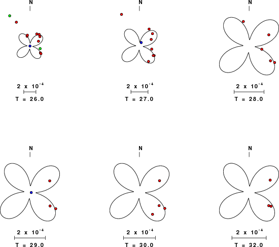
| Focal mechanism sensitivity at the preferred depth. The red color indicates a very good fit to thewavefroms. Each solution is plotted as a vector at a given value of strike and dip with the angle of the vector representing the rake angle, measured, with respect to the upward vertical (N) in the figure. |
The following figure shows the stations used in the grid search for the best focal mechanism to fit the surface-wave spectral amplitudes of the Love and Rayleigh waves.

|
|
|
The surface-wave determined focal mechanism is shown here.
  NODAL PLANES


  STK=      60.00
  DIP=      74.99
 RAKE=      54.99

             OR

  STK=     309.72
  DIP=      37.71
 RAKE=     154.96


DEPTH = 8.0 km

Mw = 3.85
Best Fit 0.8937 - P-T axis plot gives solutions with FIT greater than FIT90
 |
The P-wave first motion data for focal mechanism studies are as follow:
Sta Az(deg)    Dist(km)   First motion
U13A      253   30 -12345
U14A      102   42 -12345
T13A      338   63 -12345
V13A      203   78 -12345
T14A       38   80 -12345
U12A      265   81 -12345
T12A      285   99 -12345
V14A      153  107 -12345
CCUT       12  119 -12345
U15A       93  121 -12345
S13A      351  122 -12345
T15A       62  126 -12345
W14A      160  151 -12345
V15A      119  152 -12345
U11A      267  156 -12345
W13A      188  157 -12345
S12A      319  163 -12345
T11A      301  163 -12345
W12A      220  173 -12345
V11A      246  177 -12345
R13A      351  189 -12345
W15A      139  192 -12345
T16A       74  198 -12345
LDF       223  206 -12345
R14A       15  207 -12345
X13A      185  212 -12345
R12A      337  220 -12345
R15A       32  225 -12345
S11A      305  226 -12345
U16A       99  229 -12345
WUAZ      117  232 -12345
X14A      163  235 -12345
U10A      269  241 -12345
W16A      129  246 -12345
X15A      150  257 -12345
T17A       77  259 -12345
U17A       87  267 -12345
R11A      321  268 -12345
V17A      110  274 -12345
Q13A      353  275 -12345
Q14A        7  278 -12345
S17A       63  282 -12345
Y14A      168  290 -12345
Y13A      183  298 -12345
Q12A      340  301 -12345
X16A      138  305 -12345
S10A      302  306 -12345
Y15A      157  306 -12345
R10A      311  308 -12345
W17A      120  308 -12345
Q11A      326  315 -12345
P13A      354  330 -12345
T18A       77  343 -12345
V18A      104  345 -12345
Q16A       38  346 -12345
P12A      342  348 -12345
Y16A      145  351 -12345
Z14A      169  354 -12345
Q10A      318  355 -12345
Z15A      159  381 -12345
W18A      112  385 -12345
X18A      122  400 -12345
Y17A      140  402 -12345
Z16A      149  404 -12345
113A      182  414 -12345
W19A      111  414 -12345
DUG        10  417 -12345
114A      170  421 -12345
V19A      101  423 -12345
O12A      347  429 -12345
R19A       62  436 -12345
O11A      337  440 -12345
115A      162  441 -12345
112A      191  448 -12345
X19A      119  457 -12345
116A      157  471 -12345
N13A      354  486 -12345
W20A      107  489 -12345
ELK       344  492 -12345
BGU         6  494 -12345
Surface wave analysis was performed using codes from Computer Programs in Seismology, specifically the multiple filter analysis program do_mft and the surface-wave radiation pattern search program srfgrd96.
Digital data were collected, instrument response removed and traces converted
to Z, R an T components. Multiple filter analysis was applied to the Z and T traces to obtain the Rayleigh- and Love-wave spectral amplitudes, respectively.
These were input to the search program which examined all depths between 1 and 25 km
and all possible mechanisms.

|
|
|

|
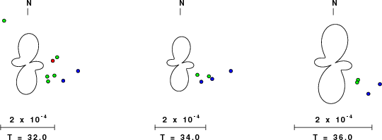
| Pressure-tension axis trends. Since the surface-wave spectra search does not distinguish between P and T axes and since there is a 180 ambiguity in strike, all possible P and T axes are plotted. First motion data and waveforms will be used to select the preferred mechanism. The purpose of this plot is to provide an idea of the possible range of solutions. The P and T-axes for all mechanisms with goodness of fit greater than 0.9 FITMAX (above) are plotted here. |

|
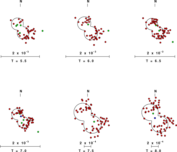
| Focal mechanism sensitivity at the preferred depth. The red color indicates a very good fit to the Love and Rayleigh wave radiation patterns. Each solution is plotted as a vector at a given value of strike and dip with the angle of the vector representing the rake angle, measured, with respect to the upward vertical (N) in the figure. Because of the symmetry of the spectral amplitude rediation patterns, only strikes from 0-180 degrees are sampled. |
The distribution of broadband stations with azimuth and distance is
Sta Az(deg)    Dist(km)
R13A	  351	  189
W15A	  139	  192
LDF	  223	  206
R14A	   15	  207
X13A	  185	  212
R12A	  337	  220
R15A	   32	  225
S11A	  305	  226
U16A	   99	  229
WUAZ	  117	  232
X14A	  163	  235
U10A	  269	  241
W16A	  129	  246
X15A	  150	  257
T17A	   77	  259
U17A	   87	  267
R11A	  321	  268
V17A	  110	  274
Q13A	  353	  275
R16A	   43	  275
Q14A	    6	  278
S17A	   63	  282
Y14A	  168	  290
Y13A	  183	  298
Q15A	   21	  299
Q12A	  340	  301
X16A	  138	  305
S10A	  302	  306
Y15A	  157	  306
R10A	  311	  308
W17A	  120	  308
GSC	  246	  315
Q11A	  326	  315
Y12C	  195	  315
P13A	  354	  330
R17A	   50	  336
U18A	   90	  338
T18A	   77	  343
V18A	  104	  345
Q16A	   38	  346
P14A	    8	  347
P12A	  342	  348
Y16A	  145	  351
Z14A	  170	  354
Q10A	  318	  355
Z13A	  180	  366
Z15A	  159	  381
R18A	   57	  392
GLA	  196	  397
U19A	   92	  398
SRU	   42	  399
X18A	  122	  400
Y17A	  140	  402
O13A	  356	  404
Z16A	  149	  404
NLU	   19	  407
113A	  182	  414
T19A	   84	  414
W19A	  111	  414
DUG	   10	  417
114A	  170	  421
Q18A	   46	  423
V19A	  100	  423
O12A	  347	  429
O15A	   13	  432
R19A	   62	  436
O11A	  337	  440
115A	  162	  441
ISA	  259	  445
112A	  191	  448
P18A	   40	  458
U20A	   90	  459
MVCO	   79	  465
116A	  157	  471
V20A	   98	  472
MWC	  239	  474
NOQ	   16	  480
O17A	   31	  482
N14A	    4	  485
N13A	  354	  486
W20A	  107	  489
Y19A	  124	  489
ELK	  344	  492
BGU	    6	  494
N15A	   11	  497
R20A	   66	  502
Z18A	  138	  502
BAR	  214	  507
117A	  148	  510
214A	  171	  510
109C	  219	  511
X20A	  113	  514
O18A	   36	  525
N10A	  333	  531
TUC	  150	  534
Z19A	  130	  535
P19A	   48	  537
216A	  157	  538
118A	  141	  545
V21A	   96	  546
N17A	   26	  550
M14A	    2	  556
M12A	  349	  557
M15A	   10	  561
W21A	  104	  563
P20A	   53	  569
O19A	   42	  577
M11A	  342	  578
X21A	  112	  578
217A	  153	  585
Z20A	  128	  595
218A	  146	  601
T22A	   83	  604
N18A	   34	  605
Y21A	  115	  609
M10A	  337	  612
L14A	    3	  616
L13A	  358	  621
L15A	   10	  621
O20A	   48	  621
N19A	   37	  623
W22A	  102	  632
120A	  132	  635
L12A	  350	  638
M09A	  330	  639
L16A	   17	  641
X22A	  108	  641
219A	  140	  642
Q22A	   64	  649
318A	  148	  655
L11A	  344	  655
L10A	  339	  666
ANMO	  103	  672
K14A	    3	  673
L18A	   26	  678
O21A	   51	  679
K13A	  357	  684
K12A	  351	  690
121A	  128	  694
220A	  136	  694
319A	  143	  696
L09A	  332	  704
L19A	   29	  723
M07A	  320	  724
K16A	   13	  725
K11A	  344	  726
M20A	   39	  728
AHID	   17	  729
K17A	   18	  732
221A	  131	  734
320A	  139	  742
K18A	   23	  748
K10A	  339	  750
J15A	    7	  773
K09A	  334	  773
222A	  127	  774
BW06	   26	  779
RRI2	   14	  786
HLID	  355	  787
WVOR	  328	  787
J11A	  347	  790
ISCO	   60	  793
REDW	   16	  798
RWWY	   42	  801
K08A	  330	  807
J10A	  342	  814
DCID1	   14	  815
M22A	   46	  818
I12A	  352	  820
LOHW	   17	  831
I15A	    6	  839
K07A	  327	  839
I11A	  347	  846
IMW	   15	  853
J08A	  333	  866
I10A	  343	  884
224A	  121	  894
H12A	  354	  900
I09A	  338	  900
H14A	    1	  902
MNTX	  123	  929
324A	  124	  939
H09A	  341	  968
BMO	  343	  978
I07A	  331	  978
325A	  123	  982
H08A	  336	  987
G11A	  348	 1013
425A	  126	 1022
G09A	  342	 1035
Since the analysis of the surface-wave radiation patterns uses only spectral amplitudes and because the surfave-wave radiation patterns have a 180 degree symmetry, each surface-wave solution consists of four possible focal mechanisms corresponding to the interchange of the P- and T-axes and a roation of the mechanism by 180 degrees. To select one mechanism, P-wave first motion can be used. This was not possible in this case because all the P-wave first motions were emergent ( a feature of the P-wave wave takeoff angle, the station location and the mechanism). The other way to select among the mechanisms is to compute forward synthetics and compare the observed and predicted waveforms.
The fits to the waveforms with the given mechanism are show below:

|
This figure shows the fit to the three components of motion (Z - vertical, R-radial and T - transverse). For each station and component, the observed traces is shown in red and the model predicted trace in blue. The traces represent filtered ground velocity in units of meters/sec (the peak value is printed adjacent to each trace; each pair of traces to plotted to the same scale to emphasize the difference in levels). Both synthetic and observed traces have been filtered using the SAC commands:
hp c 0.02 n 3
lp c 0.12 n 3
br c 0.12 0.25 n 4 p 2

|

|
Should the national backbone of the USGS Advanced National Seismic System (ANSS) be implemented with an interstation separation of 300 km, it is very likely that an earthquake such as this would have been recorded at distances on the order of 100-200 km. This means that the closest station would have information on source depth and mechanism that was lacking here.
Dr. Harley Benz, USGS, provided the USGS USNSN digital data. The digital data used in this study were provided by Natural Resources Canada through their AUTODRM site http://www.seismo.nrcan.gc.ca/nwfa/autodrm/autodrm_req_e.php, and IRIS using their BUD interface.
Thanks also to the many seismic network operators whose dedication make this effort possible: University of Alaska, University of Washington, Oregon State University, University of Utah, Montana Bureas of Mines, UC Berkely, Caltech, UC San Diego, Saint L ouis University, Universityof Memphis, Lamont Doehrty Earth Observatory, Boston College, the Iris stations and the Transportable Array of EarthScope.
The VMODEL used for the waveform synthetic seismograms and for the surface wave eigenfunctions and dispersion is as follows:
MODEL.01
Model after     8 iterations
ISOTROPIC
KGS
FLAT EARTH
1-D
CONSTANT VELOCITY
LINE08
LINE09
LINE10
LINE11
      H(KM)   VP(KM/S)   VS(KM/S) RHO(GM/CC)         QP         QS       ETAP       ETAS      FREFP      FREFS
     1.9000     3.4065     2.0089     2.2150  0.302E-02  0.679E-02   0.00       0.00       1.00       1.00
     6.1000     5.5445     3.2953     2.6089  0.349E-02  0.784E-02   0.00       0.00       1.00       1.00
    13.0000     6.2708     3.7396     2.7812  0.212E-02  0.476E-02   0.00       0.00       1.00       1.00
    19.0000     6.4075     3.7680     2.8223  0.111E-02  0.249E-02   0.00       0.00       1.00       1.00
     0.0000     7.9000     4.6200     3.2760  0.164E-10  0.370E-10   0.00       0.00       1.00       1.00
Here we tabulate the reasons for not using certain digital data sets
The following stations did not have a valid response files:
DATE=Thu Mar 27 10:34:27 CDT 2008