
2007/08/06 08:48:40 39.464 -111.218 0.0 3.8 Utah
USGS Felt map for this earthquake
 SLU Moment Tensor Solution
 2007/08/06 08:48:40 39.464 -111.218 0.0 3.8 Utah

 Best Fitting Double Couple
    Mo = 6.31e+21 dyne-cm
    Mw = 3.80
    Z  = 6 km
     Plane   Strike  Dip  Rake
      NP1      176    57   -103
      NP2       20    35   -70
 Principal Axes:
   Axis    Value   Plunge  Azimuth
     T   6.31e+21     11     276
     N   0.00e+00     11     183
     P  -6.31e+21     74      50


 Moment Tensor: (dyne-cm)
    Component  Value
       Mxx    -1.44e+20
       Mxy    -8.42e+20
       Mxz    -9.68e+20
       Myy     5.72e+21
       Myz    -2.51e+21
       Mzz    -5.57e+21


                     ####----------
                 #######-------------##
              #########----------------###
             #########------------------###
           ##########--------------------####
          ###########--------------------#####
         ###########----------------------#####
        ############----------------------######
        ############----------   ---------######
       #   #########---------- P ---------#######
       # T #########----------   ---------#######
       #   #########----------------------#######
       #############---------------------########
        ############---------------------#######
        #############-------------------########
         ############------------------########
          ############----------------########
           ############-------------#########
             ##########------------########
              ###########-------##########
                 #########---##########
                     ##-----#######


 Harvard Convention
 Moment Tensor:
      R          T          F
 -5.57e+21  -9.68e+20   2.51e+21
 -9.68e+20  -1.44e+20   8.42e+20
  2.51e+21   8.42e+20   5.72e+21


Details of the solution is found at

http://www.eas.slu.edu/eqc/eqc_mt/MECH.NA/20070806084840/index.html
|
      STK = 20
      DIP = 35
     RAKE = -70
       MW = 3.80
       HS = 6
Neither solutions is adequate because of the possibility that this event was a mine collapse. The definite characteristic of this event is the lack of low frequency signal in the waveforms. If there is a collapse which can be represented as a point force, then the source time function is approximately a one-pole high pass filter with corner period related to the tiem of free fall of the roof. If this free fall is asymmetric, then Love waves will be generated. The other way in which to remove the low frequency signal is to have a very shallow vertical dip-slip source. This event requires further study and a better background on the proper source time representation for a collapse.
The focal mechanism was determined using broadband seismic waveforms. The location of the event and the and stations used for the waveform inversion are shown in the next figure.
|
|
|
|
The program wvfgrd96 was used with good traces observed at short distance to determine the focal mechanism, depth and seismic moment. This technique requires a high quality signal and well determined velocity model for the Green functions. To the extent that these are the quality data, this type of mechanism should be preferred over the radiation pattern technique which requires the separate step of defining the pressure and tension quadrants and the correct strike.
The observed and predicted traces are filtered using the following gsac commands:
hp c 0.02 n 3
lp c 0.10 n 3
The results of this grid search from 0.5 to 19 km depth are as follow:
           DEPTH  STK   DIP  RAKE   MW    FIT
WVFGRD96    0.5   320    10   -95   3.86 0.1342
WVFGRD96    1.0   290    15   -10   3.76 0.1497
WVFGRD96    2.0   290     5   -15   3.99 0.1806
WVFGRD96    3.0   310    15   -90   3.97 0.2087
WVFGRD96    4.0   310    20   -90   3.96 0.2121
WVFGRD96    5.0   315    30   -90   3.96 0.2010
WVFGRD96    6.0   310    30   -95   3.95 0.1850
WVFGRD96    7.0    35    50    65   3.91 0.1648
WVFGRD96    8.0   140    55   -85   4.00 0.1436
WVFGRD96    9.0   145    55   -80   3.98 0.1252
WVFGRD96   10.0   150    50   -70   3.97 0.1083
WVFGRD96   11.0    25    55    45   3.92 0.0950
WVFGRD96   12.0   165    40   -50   3.95 0.0842
WVFGRD96   13.0   165    40   -45   3.94 0.0759
WVFGRD96   14.0   170    40   -40   3.94 0.0690
WVFGRD96   15.0   170    40   -40   3.94 0.0628
WVFGRD96   16.0   170    40   -40   3.95 0.0577
WVFGRD96   17.0    90    25    40   3.94 0.0537
WVFGRD96   18.0   190    60    35   3.92 0.0511
WVFGRD96   19.0   195    60    35   3.93 0.0500
WVFGRD96   20.0   195    60    35   3.94 0.0494
WVFGRD96   21.0   195    60    35   3.95 0.0492
WVFGRD96   22.0   195    60    40   3.96 0.0490
WVFGRD96   23.0   195    60    40   3.97 0.0489
WVFGRD96   24.0   200    55    45   3.97 0.0489
WVFGRD96   25.0   200    55    45   3.98 0.0483
WVFGRD96   26.0   200    60    45   3.99 0.0478
WVFGRD96   27.0   115    30    65   4.04 0.0476
WVFGRD96   28.0   320    65   -75   4.05 0.0476
WVFGRD96   29.0   205    65    45   4.01 0.0480
The best solution is
WVFGRD96 4.0 310 20 -90 3.96 0.2121
The mechanism correspond to the best fit is

|
|
|
The best fit as a function of depth is given in the following figure:

|
|
|
The comparison of the observed and predicted waveforms is given in the next figure. The red traces are the observed and the blue are the predicted. Each observed-predicted componnet is plotted to the same scale and peak amplitudes are indicated by the numbers to the left of each trace. The number in black at the rightr of each predicted traces it the time shift required for maximum correlation between the observed and predicted traces. This time shift is required because the synthetics are not computed at exactly the same distance as the observed and because the velocity model used in the predictions may not be perfect. A positive time shift indicates that the prediction is too fast and should be delayed to match the observed trace (shift to the right in this figure). A negative value indicates that the prediction is too slow. The bandpass filter used in the processing and for the display was
hp c 0.02 n 3
lp c 0.10 n 3

|
|
|

|
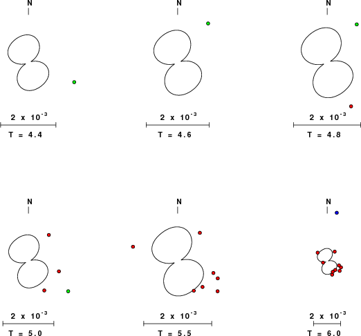
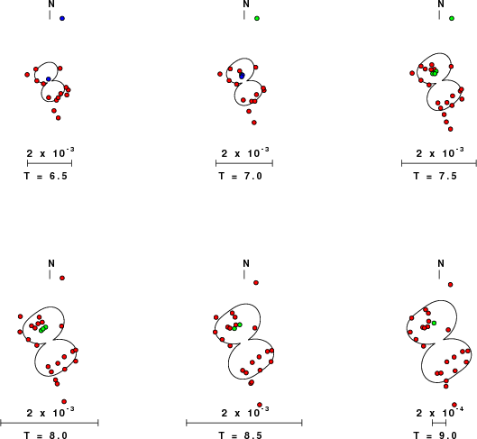
| Focal mechanism sensitivity at the preferred depth. The red color indicates a very good fit to thewavefroms. Each solution is plotted as a vector at a given value of strike and dip with the angle of the vector representing the rake angle, measured, with respect to the upward vertical (N) in the figure. |
The following figure shows the stations used in the grid search for the best focal mechanism to fit the surface-wave spectral amplitudes of the Love and Rayleigh waves.

|
|
|
The surface-wave determined focal mechanism is shown here.
  NODAL PLANES


  STK=     340.50
  DIP=      75.52
 RAKE=      93.96

             OR

  STK=     145.01
  DIP=      15.00
 RAKE=      75.01


DEPTH = 6.0 km

Mw = 3.95
Best Fit 0.7428 - P-T axis plot gives solutions with FIT greater than FIT90
 |
The P-wave first motion data for focal mechanism studies are as follow:
Sta Az(deg)    Dist(km)   First motion
TMU       177   19 eP_X
P16A      293   41 iP_D
P17A       88   41 eP_-
Q16A      176   61 eP_-
MPU       330   71 eP_X
SRU       123   72 iP_D
O16A      344   86 iP_-
P18A       77   86 eP_-
NLU       307   91 iP_D
P15A      278   92 iP_-
Q18A      113  102 iP_-
Q15A      243  113 eP_X
R17A      159  124 iP_D
O18A       49  137 iP_D
O15A      311  140 iP_D
DUG       301  159 iP_D
N16A      353  159 iP_D
P14A      276  160 iP_D
N17A       11  167 eP_-
R15A      214  167 iP_D
MVCO      136  345 eP_-
AHID        2  367 eP_X
ELK       294  371 eP_X
BW06       20  392 eP_-
REDW        4  434 iP_C
WUAZ      182  438 eP_-
ISCO       84  483 eP_X
Surface wave analysis was performed using codes from Computer Programs in Seismology, specifically the multiple filter analysis program do_mft and the surface-wave radiation pattern search program srfgrd96.
Digital data were collected, instrument response removed and traces converted
to Z, R an T components. Multiple filter analysis was applied to the Z and T traces to obtain the Rayleigh- and Love-wave spectral amplitudes, respectively.
These were input to the search program which examined all depths between 1 and 25 km
and all possible mechanisms.

|
|
|

|
| Pressure-tension axis trends. Since the surface-wave spectra search does not distinguish between P and T axes and since there is a 180 ambiguity in strike, all possible P and T axes are plotted. First motion data and waveforms will be used to select the preferred mechanism. The purpose of this plot is to provide an idea of the possible range of solutions. The P and T-axes for all mechanisms with goodness of fit greater than 0.9 FITMAX (above) are plotted here. |

|
| Focal mechanism sensitivity at the preferred depth. The red color indicates a very good fit to the Love and Rayleigh wave radiation patterns. Each solution is plotted as a vector at a given value of strike and dip with the angle of the vector representing the rake angle, measured, with respect to the upward vertical (N) in the figure. Because of the symmetry of the spectral amplitude rediation patterns, only strikes from 0-180 degrees are sampled. |
The distribution of broadband stations with azimuth and distance is
Sta Az(deg)    Dist(km)
P17A	   88	   41
Q16A	  176	   61
O16A	  344	   86
P18A	   77	   86
P15A	  278	   92
Q18A	  113	  102
Q15A	  243	  113
R17A	  159	  124
O18A	   49	  137
O15A	  311	  140
N16A	  353	  159
P14A	  276	  160
R18A	  136	  166
N17A	   11	  167
R15A	  214	  167
Q19A	  108	  178
Q14A	  254	  185
S17A	  170	  206
N18A	   38	  213
R19A	  127	  214
S18A	  151	  224
N14A	  313	  228
O13A	  288	  248
H13A	  337	  620
H12A	  333	  640
G15A	  351	  642
G14A	  345	  668
G13A	  339	  673
H11A	  327	  704
H10A	  323	  730
F13A	  341	  747
119A	  166	  763
118A	  171	  765
117A	  177	  766
116A	  183	  767
E15A	  352	  782
I08A	  311	  786
318A	  172	  897
Since the analysis of the surface-wave radiation patterns uses only spectral amplitudes and because the surfave-wave radiation patterns have a 180 degree symmetry, each surface-wave solution consists of four possible focal mechanisms corresponding to the interchange of the P- and T-axes and a roation of the mechanism by 180 degrees. To select one mechanism, P-wave first motion can be used. This was not possible in this case because all the P-wave first motions were emergent ( a feature of the P-wave wave takeoff angle, the station location and the mechanism). The other way to select among the mechanisms is to compute forward synthetics and compare the observed and predicted waveforms.
The fits to the waveforms with the given mechanism are show below:

|
This figure shows the fit to the three components of motion (Z - vertical, R-radial and T - transverse). For each station and component, the observed traces is shown in red and the model predicted trace in blue. The traces represent filtered ground velocity in units of meters/sec (the peak value is printed adjacent to each trace; each pair of traces to plotted to the same scale to emphasize the difference in levels). Both synthetic and observed traces have been filtered using the SAC commands:
hp c 0.02 n 3
lp c 0.10 n 3
br c 0.12 0.25 n 4 p 2

|

|
Should the national backbone of the USGS Advanced National Seismic System (ANSS) be implemented with an interstation separation of 300 km, it is very likely that an earthquake such as this would have been recorded at distances on the order of 100-200 km. This means that the closest station would have information on source depth and mechanism that was lacking here.
Dr. Harley Benz, USGS, provided the USGS USNSN digital data. The digital data used in this study were provided by Natural Resources Canada through their AUTODRM site http://www.seismo.nrcan.gc.ca/nwfa/autodrm/autodrm_req_e.php, and IRIS using their BUD interface
The WUS used for the waveform synthetic seismograms and for the surface wave eigenfunctions and dispersion is as follows:
MODEL.01
Model after     8 iterations
ISOTROPIC
KGS
FLAT EARTH
1-D
CONSTANT VELOCITY
LINE08
LINE09
LINE10
LINE11
      H(KM)   VP(KM/S)   VS(KM/S) RHO(GM/CC)         QP         QS       ETAP       ETAS      FREFP      FREFS
     1.9000     3.4065     2.0089     2.2150  0.302E-02  0.679E-02   0.00       0.00       1.00       1.00
     6.1000     5.5445     3.2953     2.6089  0.349E-02  0.784E-02   0.00       0.00       1.00       1.00
    13.0000     6.2708     3.7396     2.7812  0.212E-02  0.476E-02   0.00       0.00       1.00       1.00
    19.0000     6.4075     3.7680     2.8223  0.111E-02  0.249E-02   0.00       0.00       1.00       1.00
     0.0000     7.9000     4.6200     3.2760  0.164E-10  0.370E-10   0.00       0.00       1.00       1.00
Here we tabulate the reasons for not using certain digital data sets
The following stations did not have a valid response files:
DATE=Tue Aug 7 21:51:48 CDT 2007