
2007/06/11 01:03:46 37.50 -114.04 0 3.9 Utah
USGS Felt map for this earthquake
 USGS/SLU Moment Tensor Solution
 ENS  2007/06/11 01:03:46:0  37.50 -114.04   0.0 3.9 Utah

 Stations used:
   AZ.KNW CI.BC3 CI.CHF CI.CWC CI.FUR CI.GLA CI.GMR CI.GRA
   CI.GSC CI.MLAC CI.MPM CI.MWC CI.PASC CI.RCT CI.SHO CI.SLA
   CI.TIN CI.TUQ CI.VES II.PFO IM.NV31 LB.TPH TA.113A TA.HELL
   TA.L11A TA.L12A TA.L13A TA.M11A TA.M14A TA.M15A TA.N08A
   TA.N12A TA.N13A TA.N14A TA.O07A TA.O08A TA.O09A TA.O10A
   TA.O11A TA.O12A TA.O13A TA.P10A TA.P12A TA.P13A TA.P15A
   TA.P16A TA.Q08A TA.Q12A TA.Q13A TA.Q16A TA.R06C TA.R08A
   TA.R09A TA.R10A TA.R11A TA.R13A TA.R14A TA.R15A TA.S06C
   TA.S08C TA.S09A TA.S10A TA.S11A TA.S12A TA.S14A TA.S15A
   TA.T06C TA.T11A TA.T13A TA.T15A TA.T16A TA.U10A TA.U11A
   TA.U13A TA.U14A TA.U15A TA.U17A TA.V14A TA.V15A TA.W12A
   TA.W13A TA.W14A TA.W16A TA.W18A TA.W19A TA.X13A TA.X14A
   TA.Y13A TA.Y14A TA.Y15A TA.Y16A TA.Y18A TA.Z14A US.DUG
   US.MVCO US.TPNV UU.BGU UU.CCUT UU.SRU XE.SNP63 XE.SNP75

 Filtering commands used:
   cut a -30 a 180
   rtr
   taper w 0.1
   hp c 0.02 n 3
   lp c 0.06 n 3

 Best Fitting Double Couple
  Mo = 5.13e+21 dyne-cm
  Mw = 3.74
  Z  = 9 km
  Plane   Strike  Dip  Rake
   NP1      345    90   -155
   NP2      255    65     0
  Principal Axes:
   Axis    Value   Plunge  Azimuth
    T   5.13e+21     17     117
    N   0.00e+00     65     345
    P  -5.13e+21     17     213

 Moment Tensor: (dyne-cm)
    Component   Value
       Mxx    -2.32e+21
       Mxy    -4.03e+21
       Mxz     5.61e+20
       Myy     2.32e+21
       Myz     2.09e+21
       Mzz     0.00e+00


                     ##------------
                 ######----------------
              ##########------------------
             ###########-------------------
           ##############--------------------
          ###############---------------------
         #################---------------------
        ##################--#################---
        ##############-----#####################
       ###########---------######################
       #######--------------#####################
       #####----------------#####################
       ###-------------------####################
        ---------------------###################
        ----------------------############   ###
         ---------------------############ T ##
          ---------------------###########   #
           ------   -----------##############
             ---- P ------------###########
              ---   ------------##########
                 ----------------######
                     ------------##


 Global CMT Convention Moment Tensor:
      R          T          P
  0.00e+00   5.61e+20  -2.09e+21
  5.61e+20  -2.32e+21   4.03e+21
 -2.09e+21   4.03e+21   2.32e+21


Details of the solution is found at

http://www.eas.slu.edu/eqc/eqc_mt/MECH.NA/20070611010346/index.html
|
      STK = 255
      DIP = 65
     RAKE = 0
       MW = 3.74
       HS = 9.0
The NDK file is 20070611010346.ndk The waveform inversion is preferred.
The following compares this source inversion to others
 USGS/SLU Moment Tensor Solution
 ENS  2007/06/11 01:03:46:0  37.50 -114.04   0.0 3.9 Utah

 Stations used:
   AZ.KNW CI.BC3 CI.CHF CI.CWC CI.FUR CI.GLA CI.GMR CI.GRA
   CI.GSC CI.MLAC CI.MPM CI.MWC CI.PASC CI.RCT CI.SHO CI.SLA
   CI.TIN CI.TUQ CI.VES II.PFO IM.NV31 LB.TPH TA.113A TA.HELL
   TA.L11A TA.L12A TA.L13A TA.M11A TA.M14A TA.M15A TA.N08A
   TA.N12A TA.N13A TA.N14A TA.O07A TA.O08A TA.O09A TA.O10A
   TA.O11A TA.O12A TA.O13A TA.P10A TA.P12A TA.P13A TA.P15A
   TA.P16A TA.Q08A TA.Q12A TA.Q13A TA.Q16A TA.R06C TA.R08A
   TA.R09A TA.R10A TA.R11A TA.R13A TA.R14A TA.R15A TA.S06C
   TA.S08C TA.S09A TA.S10A TA.S11A TA.S12A TA.S14A TA.S15A
   TA.T06C TA.T11A TA.T13A TA.T15A TA.T16A TA.U10A TA.U11A
   TA.U13A TA.U14A TA.U15A TA.U17A TA.V14A TA.V15A TA.W12A
   TA.W13A TA.W14A TA.W16A TA.W18A TA.W19A TA.X13A TA.X14A
   TA.Y13A TA.Y14A TA.Y15A TA.Y16A TA.Y18A TA.Z14A US.DUG
   US.MVCO US.TPNV UU.BGU UU.CCUT UU.SRU XE.SNP63 XE.SNP75

 Filtering commands used:
   cut a -30 a 180
   rtr
   taper w 0.1
   hp c 0.02 n 3
   lp c 0.06 n 3

 Best Fitting Double Couple
  Mo = 5.13e+21 dyne-cm
  Mw = 3.74
  Z  = 9 km
  Plane   Strike  Dip  Rake
   NP1      345    90   -155
   NP2      255    65     0
  Principal Axes:
   Axis    Value   Plunge  Azimuth
    T   5.13e+21     17     117
    N   0.00e+00     65     345
    P  -5.13e+21     17     213

 Moment Tensor: (dyne-cm)
    Component   Value
       Mxx    -2.32e+21
       Mxy    -4.03e+21
       Mxz     5.61e+20
       Myy     2.32e+21
       Myz     2.09e+21
       Mzz     0.00e+00


                     ##------------
                 ######----------------
              ##########------------------
             ###########-------------------
           ##############--------------------
          ###############---------------------
         #################---------------------
        ##################--#################---
        ##############-----#####################
       ###########---------######################
       #######--------------#####################
       #####----------------#####################
       ###-------------------####################
        ---------------------###################
        ----------------------############   ###
         ---------------------############ T ##
          ---------------------###########   #
           ------   -----------##############
             ---- P ------------###########
              ---   ------------##########
                 ----------------######
                     ------------##


 Global CMT Convention Moment Tensor:
      R          T          P
  0.00e+00   5.61e+20  -2.09e+21
  5.61e+20  -2.32e+21   4.03e+21
 -2.09e+21   4.03e+21   2.32e+21


Details of the solution is found at

http://www.eas.slu.edu/eqc/eqc_mt/MECH.NA/20070611010346/index.html
|
The focal mechanism was determined using broadband seismic waveforms. The location of the event and the and stations used for the waveform inversion are shown in the next figure.
|
|
|
|
The program wvfgrd96 was used with good traces observed at short distance to determine the focal mechanism, depth and seismic moment. This technique requires a high quality signal and well determined velocity model for the Green functions. To the extent that these are the quality data, this type of mechanism should be preferred over the radiation pattern technique which requires the separate step of defining the pressure and tension quadrants and the correct strike.
The observed and predicted traces are filtered using the following gsac commands:
cut a -30 a 180
rtr
taper w 0.1
hp c 0.02 n 3
lp c 0.06 n 3
The results of this grid search from 0.5 to 19 km depth are as follow:
           DEPTH  STK   DIP  RAKE   MW    FIT
WVFGRD96    1.0    70    85   -10   3.43 0.3158
WVFGRD96    2.0   250    75   -15   3.54 0.4020
WVFGRD96    3.0   250    60   -10   3.61 0.4395
WVFGRD96    4.0   250    60   -10   3.64 0.4694
WVFGRD96    5.0   250    65   -10   3.66 0.4902
WVFGRD96    6.0   250    65   -10   3.68 0.5056
WVFGRD96    7.0   255    70     0   3.69 0.5167
WVFGRD96    8.0   255    65     0   3.72 0.5253
WVFGRD96    9.0   255    65     0   3.74 0.5283
WVFGRD96   10.0   255    65     5   3.75 0.5279
WVFGRD96   11.0   255    70     5   3.76 0.5255
WVFGRD96   12.0   255    70     5   3.77 0.5219
WVFGRD96   13.0   255    70     5   3.78 0.5172
WVFGRD96   14.0   255    70     5   3.79 0.5109
WVFGRD96   15.0   255    70     5   3.79 0.5040
WVFGRD96   16.0   255    70     5   3.80 0.4966
WVFGRD96   17.0   255    70     5   3.81 0.4886
WVFGRD96   18.0   255    70     5   3.81 0.4802
WVFGRD96   19.0   255    75    10   3.82 0.4720
WVFGRD96   20.0   255    75    10   3.83 0.4642
WVFGRD96   21.0   255    75    10   3.84 0.4562
WVFGRD96   22.0   255    75    10   3.84 0.4482
WVFGRD96   23.0   255    75    10   3.85 0.4401
WVFGRD96   24.0   255    75    10   3.85 0.4320
WVFGRD96   25.0   255    75    10   3.86 0.4237
WVFGRD96   26.0   255    75     5   3.86 0.4158
WVFGRD96   27.0   255    75     5   3.87 0.4081
WVFGRD96   28.0   255    75     5   3.87 0.4006
WVFGRD96   29.0   255    75     5   3.88 0.3932
The best solution is
WVFGRD96 9.0 255 65 0 3.74 0.5283
The mechanism correspond to the best fit is

|
|
|
The best fit as a function of depth is given in the following figure:

|
|
|
The comparison of the observed and predicted waveforms is given in the next figure. The red traces are the observed and the blue are the predicted. Each observed-predicted component is plotted to the same scale and peak amplitudes are indicated by the numbers to the left of each trace. A pair of numbers is given in black at the right of each predicted traces. The upper number it the time shift required for maximum correlation between the observed and predicted traces. This time shift is required because the synthetics are not computed at exactly the same distance as the observed and because the velocity model used in the predictions may not be perfect. A positive time shift indicates that the prediction is too fast and should be delayed to match the observed trace (shift to the right in this figure). A negative value indicates that the prediction is too slow. The lower number gives the percentage of variance reduction to characterize the individual goodness of fit (100% indicates a perfect fit).
The bandpass filter used in the processing and for the display was
cut a -30 a 180
rtr
taper w 0.1
hp c 0.02 n 3
lp c 0.06 n 3

|
|
|

|
| Focal mechanism sensitivity at the preferred depth. The red color indicates a very good fit to thewavefroms. Each solution is plotted as a vector at a given value of strike and dip with the angle of the vector representing the rake angle, measured, with respect to the upward vertical (N) in the figure. |
A check on the assumed source location is possible by looking at the time shifts between the observed and predicted traces. The time shifts for waveform matching arise for several reasons:
Time_shift = A + B cos Azimuth + C Sin Azimuth
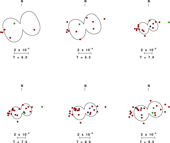
The time shifts for this inversion lead to the next figure:

The derived shift in origin time and epicentral coordinates are given at the bottom of the figure.
The following figure shows the stations used in the grid search for the best focal mechanism to fit the surface-wave spectral amplitudes of the Love and Rayleigh waves.

|
|
|
The surface-wave determined focal mechanism is shown here.
  NODAL PLANES


  STK=     157.87
  DIP=      85.47
 RAKE=     154.92

             OR

  STK=     249.98
  DIP=      65.00
 RAKE=       5.00


DEPTH = 9.0 km

Mw = 3.81
Best Fit 0.8809 - P-T axis plot gives solutions with FIT greater than FIT90
 |
The P-wave first motion data for focal mechanism studies are as follow:
Sta Az Dist First motion
Surface wave analysis was performed using codes from Computer Programs in Seismology, specifically the multiple filter analysis program do_mft and the surface-wave radiation pattern search program srfgrd96.
Digital data were collected, instrument response removed and traces converted
to Z, R an T components. Multiple filter analysis was applied to the Z and T traces to obtain the Rayleigh- and Love-wave spectral amplitudes, respectively.
These were input to the search program which examined all depths between 1 and 25 km
and all possible mechanisms.

|
|
|

|
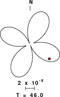
| Pressure-tension axis trends. Since the surface-wave spectra search does not distinguish between P and T axes and since there is a 180 ambiguity in strike, all possible P and T axes are plotted. First motion data and waveforms will be used to select the preferred mechanism. The purpose of this plot is to provide an idea of the possible range of solutions. The P and T-axes for all mechanisms with goodness of fit greater than 0.9 FITMAX (above) are plotted here. |

|
| Focal mechanism sensitivity at the preferred depth. The red color indicates a very good fit to the Love and Rayleigh wave radiation patterns. Each solution is plotted as a vector at a given value of strike and dip with the angle of the vector representing the rake angle, measured, with respect to the upward vertical (N) in the figure. Because of the symmetry of the spectral amplitude rediation patterns, only strikes from 0-180 degrees are sampled. |
The distribution of broadband stations with azimuth and distance is
Listing of broadband stations used
Since the analysis of the surface-wave radiation patterns uses only spectral amplitudes and because the surfave-wave radiation patterns have a 180 degree symmetry, each surface-wave solution consists of four possible focal mechanisms corresponding to the interchange of the P- and T-axes and a roation of the mechanism by 180 degrees. To select one mechanism, P-wave first motion can be used. This was not possible in this case because all the P-wave first motions were emergent ( a feature of the P-wave wave takeoff angle, the station location and the mechanism). The other way to select among the mechanisms is to compute forward synthetics and compare the observed and predicted waveforms.
The fits to the waveforms with the given mechanism are show below:

|
This figure shows the fit to the three components of motion (Z - vertical, R-radial and T - transverse). For each station and component, the observed traces is shown in red and the model predicted trace in blue. The traces represent filtered ground velocity in units of meters/sec (the peak value is printed adjacent to each trace; each pair of traces to plotted to the same scale to emphasize the difference in levels). Both synthetic and observed traces have been filtered using the SAC commands:
cut a -30 a 180
rtr
taper w 0.1
hp c 0.02 n 3
lp c 0.06 n 3

|

|
Thanks also to the many seismic network operators whose dedication make this effort possible: University of Nevada Reno, University of Alaska, University of Washington, Oregon State University, University of Utah, Montana Bureas of Mines, UC Berkely, Caltech, UC San Diego, Saint Louis University, University of Memphis, Lamont Doherty Earth Observatory, the Iris stations and the Transportable Array of EarthScope.
The WUS.model used for the waveform synthetic seismograms and for the surface wave eigenfunctions and dispersion is as follows:
MODEL.01
Model after     8 iterations
ISOTROPIC
KGS
FLAT EARTH
1-D
CONSTANT VELOCITY
LINE08
LINE09
LINE10
LINE11
      H(KM)   VP(KM/S)   VS(KM/S) RHO(GM/CC)         QP         QS       ETAP       ETAS      FREFP      FREFS
     1.9000     3.4065     2.0089     2.2150  0.302E-02  0.679E-02   0.00       0.00       1.00       1.00
     6.1000     5.5445     3.2953     2.6089  0.349E-02  0.784E-02   0.00       0.00       1.00       1.00
    13.0000     6.2708     3.7396     2.7812  0.212E-02  0.476E-02   0.00       0.00       1.00       1.00
    19.0000     6.4075     3.7680     2.8223  0.111E-02  0.249E-02   0.00       0.00       1.00       1.00
     0.0000     7.9000     4.6200     3.2760  0.164E-10  0.370E-10   0.00       0.00       1.00       1.00
Here we tabulate the reasons for not using certain digital data sets
The following stations did not have a valid response files: