
2007/06/09 10:45:44 36.93N 104.79W 1 3.3 New Mexico
USGS Felt map for this earthquake
USGS Felt reports page for Central and Southeastern US
 SLU Moment Tensor Solution
 2007/06/09 10:45:44 36.93N 104.79W 1 3.3 New Mexico

 Best Fitting Double Couple
    Mo = 1.33e+21 dyne-cm
    Mw = 3.35
    Z  = 4 km
     Plane   Strike  Dip  Rake
      NP1      195    50   -60
      NP2      333    48   -121
 Principal Axes:
   Axis    Value   Plunge  Azimuth
     T   1.33e+21      1     264
     N   0.00e+00     23     355
     P  -1.33e+21     67     172


 Moment Tensor: (dyne-cm)
    Component  Value
       Mxx    -1.79e+20
       Mxy     1.58e+20
       Mxz     4.66e+20
       Myy     1.32e+21
       Myz    -8.28e+19
       Mzz    -1.14e+21


                     -----------###
                 ######-----###########
              ############-###############
             ###########------#############
           ############---------#############
          ###########-------------############
         ###########---------------############
        ############----------------############
        ###########------------------###########
       ###########--------------------###########
       ###########---------------------##########
         #########---------------------##########
       T ########----------   ----------#########
         ########---------- P ----------########
        #########----------   ----------########
         ########-----------------------#######
          ########----------------------######
           #######----------------------#####
             ######---------------------###
              ######-------------------###
                 ####-----------------#
                     #-------------


 Harvard Convention
 Moment Tensor:
      R          T          F
 -1.14e+21   4.66e+20   8.28e+19
  4.66e+20  -1.79e+20  -1.58e+20
  8.28e+19  -1.58e+20   1.32e+21


Details of the solution is found at

http://www.eas.slu.edu/eqc/eqc_mt/MECH.NA/20070609104544/index.html
|
      STK = 195
      DIP = 50
     RAKE = -60
       MW = 3.35
       HS = 4
This a marginal event which had some good signals. The waveforms inversion is preferred. The moment is OK but hte depth is not well determined.
The focal mechanism was determined using broadband seismic waveforms. The location of the event and the and stations used for the waveform inversion are shown in the next figure.
|
|
|
|
The program wvfgrd96 was used with good traces observed at short distance to determine the focal mechanism, depth and seismic moment. This technique requires a high quality signal and well determined velocity model for the Green functions. To the extent that these are the quality data, this type of mechanism should be preferred over the radiation pattern technique which requires the separate step of defining the pressure and tension quadrants and the correct strike.
The observed and predicted traces are filtered using the following gsac commands:
hp c 0.025 n 3
lp c 0.06 n 3
br c 0.12 0.25 n 4 p 2
The results of this grid search from 0.5 to 19 km depth are as follow:
           DEPTH  STK   DIP  RAKE   MW    FIT
WVFGRD96    0.5   210    30   -20   3.32 0.2225
WVFGRD96    1.0   210    30   -20   3.34 0.2262
WVFGRD96    2.0   205    50   -40   3.26 0.2330
WVFGRD96    3.0   200    50   -50   3.31 0.2452
WVFGRD96    4.0   195    50   -60   3.35 0.2532
WVFGRD96    5.0   185    45   -75   3.40 0.2488
WVFGRD96    6.0   155    40  -100   3.38 0.2376
WVFGRD96    7.0    35    65    50   3.30 0.2345
WVFGRD96    8.0    30    70    45   3.28 0.2360
WVFGRD96    9.0    35    70    45   3.29 0.2362
WVFGRD96   10.0    35    70    45   3.30 0.2365
WVFGRD96   11.0    30    75    40   3.29 0.2373
WVFGRD96   12.0    30    75    40   3.29 0.2380
WVFGRD96   13.0    30    75    40   3.30 0.2378
WVFGRD96   14.0    30    75    40   3.30 0.2369
WVFGRD96   15.0    30    75    35   3.30 0.2359
WVFGRD96   16.0    30    75    35   3.31 0.2346
WVFGRD96   17.0    25    80    35   3.31 0.2334
WVFGRD96   18.0    25    80    35   3.31 0.2320
WVFGRD96   19.0    25    80    35   3.32 0.2305
The best solution is
WVFGRD96 4.0 195 50 -60 3.35 0.2532
The mechanism correspond to the best fit is

|
|
|
The best fit as a function of depth is given in the following figure:

|
|
|
The comparison of the observed and predicted waveforms is given in the next figure. The red traces are the observed and the blue are the predicted. Each observed-predicted componnet is plotted to the same scale and peak amplitudes are indicated by the numbers to the left of each trace. The number in black at the rightr of each predicted traces it the time shift required for maximum correlation between the observed and predicted traces. This time shift is required because the synthetics are not computed at exactly the same distance as the observed and because the velocity model used in the predictions may not be perfect. A positive time shift indicates that the prediction is too fast and should be delayed to match the observed trace (shift to the right in this figure). A negative value indicates that the prediction is too slow. The bandpass filter used in the processing and for the display was
hp c 0.025 n 3
lp c 0.06 n 3
br c 0.12 0.25 n 4 p 2

|
|
|

|
| Focal mechanism sensitivity at the preferred depth. The red color indicates a very good fit to thewavefroms. Each solution is plotted as a vector at a given value of strike and dip with the angle of the vector representing the rake angle, measured, with respect to the upward vertical (N) in the figure. |
The following figure shows the stations used in the grid search for the best focal mechanism to fit the surface-wave spectral amplitudes of the Love and Rayleigh waves.

|
|
|
The surface-wave determined focal mechanism is shown here.
  NODAL PLANES


  STK=     175.15
  DIP=      60.21
 RAKE=     -70.70

             OR

  STK=     319.97
  DIP=      35.00
 RAKE=    -120.00


DEPTH = 5.0 km

Mw = 3.46
Best Fit 0.8945 - P-T axis plot gives solutions with FIT greater than FIT90
 |
The P-wave first motion data for focal mechanism studies are as follow:
Sta Az(deg)    Dist(km)   First motion
ANMO      215  267 eP_-
SMCO      323  315 eP_X
ISCO      348  327 eP_X
MVCO      276  331 eP_X
AMTX      128  361 eP_X
CBKS       63  491 iP_D
Surface wave analysis was performed using codes from Computer Programs in Seismology, specifically the multiple filter analysis program do_mft and the surface-wave radiation pattern search program srfgrd96.
Digital data were collected, instrument response removed and traces converted
to Z, R an T components. Multiple filter analysis was applied to the Z and T traces to obtain the Rayleigh- and Love-wave spectral amplitudes, respectively.
These were input to the search program which examined all depths between 1 and 25 km
and all possible mechanisms.

|
|
|

|
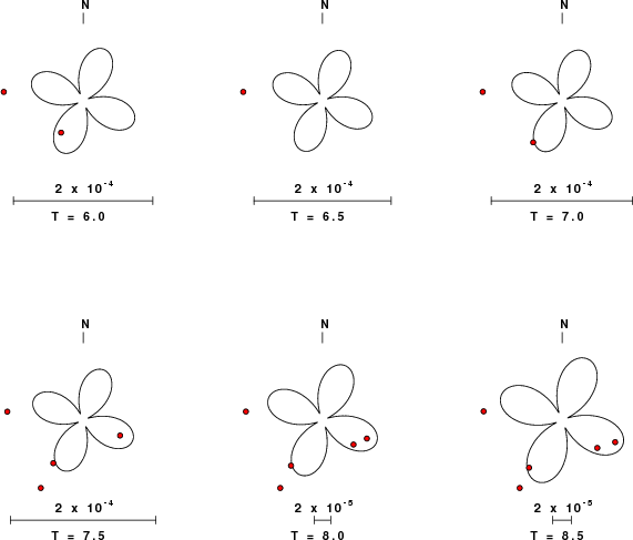
| Pressure-tension axis trends. Since the surface-wave spectra search does not distinguish between P and T axes and since there is a 180 ambiguity in strike, all possible P and T axes are plotted. First motion data and waveforms will be used to select the preferred mechanism. The purpose of this plot is to provide an idea of the possible range of solutions. The P and T-axes for all mechanisms with goodness of fit greater than 0.9 FITMAX (above) are plotted here. |

|
| Focal mechanism sensitivity at the preferred depth. The red color indicates a very good fit to the Love and Rayleigh wave radiation patterns. Each solution is plotted as a vector at a given value of strike and dip with the angle of the vector representing the rake angle, measured, with respect to the upward vertical (N) in the figure. Because of the symmetry of the spectral amplitude rediation patterns, only strikes from 0-180 degrees are sampled. |
The distribution of broadband stations with azimuth and distance is
Sta Az(deg)    Dist(km)
ANMO	  215	  267
ISCO	  348	  327
MVCO	  276	  331
AMTX	  128	  361
Y22C	  212	  371
V19A	  252	  405
U18A	  264	  458
W19A	  245	  461
V18A	  255	  481
W18A	  247	  489
SRU	  297	  558
U16A	  263	  574
Z19A	  227	  574
MNTX	  186	  583
Y18A	  235	  591
WMOK	  112	  595
Q16A	  293	  603
TUC	  229	  751
DUG	  300	  787
ECSD	   40	 1026
MIAR	  101	 1048
CCM	   80	 1203
Since the analysis of the surface-wave radiation patterns uses only spectral amplitudes and because the surfave-wave radiation patterns have a 180 degree symmetry, each surface-wave solution consists of four possible focal mechanisms corresponding to the interchange of the P- and T-axes and a roation of the mechanism by 180 degrees. To select one mechanism, P-wave first motion can be used. This was not possible in this case because all the P-wave first motions were emergent ( a feature of the P-wave wave takeoff angle, the station location and the mechanism). The other way to select among the mechanisms is to compute forward synthetics and compare the observed and predicted waveforms.
The fits to the waveforms with the given mechanism are show below:

|
This figure shows the fit to the three components of motion (Z - vertical, R-radial and T - transverse). For each station and component, the observed traces is shown in red and the model predicted trace in blue. The traces represent filtered ground velocity in units of meters/sec (the peak value is printed adjacent to each trace; each pair of traces to plotted to the same scale to emphasize the difference in levels). Both synthetic and observed traces have been filtered using the SAC commands:
hp c 0.025 n 3
lp c 0.06 n 3
br c 0.12 0.25 n 4 p 2

|

|
Should the national backbone of the USGS Advanced National Seismic System (ANSS) be implemented with an interstation separation of 300 km, it is very likely that an earthquake such as this would have been recorded at distances on the order of 100-200 km. This means that the closest station would have information on source depth and mechanism that was lacking here.
Dr. Harley Benz, USGS, provided the USGS USNSN digital data. The digital data used in this study were provided by Natural Resources Canada through their AUTODRM site http://www.seismo.nrcan.gc.ca/nwfa/autodrm/autodrm_req_e.php, and IRIS using their BUD interface
Here we tabulate the reasons for not using certain digital data sets
The following stations did not have a valid response files: