
2007/03/29 05:39:31 45.34N 112.58W 13. 3.7 Montana
USGS Felt map for this earthquake
USGS Felt reports page for Intermountain Western US
 SLU Moment Tensor Solution
 2007/03/29 05:39:31 45.34N 112.58W  13. 3.7 Montana

 Best Fitting Double Couple
    Mo = 4.62e+21 dyne-cm
    Mw = 3.71
    Z  = 11 km
     Plane   Strike  Dip  Rake
      NP1        5    50   -60
      NP2      143    48   -121
 Principal Axes:
   Axis    Value   Plunge  Azimuth
     T   4.62e+21      1      74
     N   0.00e+00     23     165
     P  -4.62e+21     67     342


 Moment Tensor: (dyne-cm)
    Component  Value
       Mxx    -2.78e+20
       Mxy     1.40e+21
       Mxz    -1.54e+21
       Myy     4.22e+21
       Myz     5.63e+20
       Mzz    -3.94e+21


                     ----------####
                 ----------------######
              #-------------------########
             ##--------------------########
           ###----------------------#########
          ####-----------------------#########
         #####-----------------------#########
        ######-----------   ----------######## T
        #######---------- P ----------########
       ########----------   ----------###########
       #########----------------------###########
       #########----------------------###########
       ##########---------------------###########
        ###########------------------###########
        ############-----------------###########
         ############---------------###########
          #############-------------##########
           ##############----------##########
             ###############------#########
              ############################
                 ##############--------
                     #######-------


 Harvard Convention
 Moment Tensor:
      R          T          F
 -3.94e+21  -1.54e+21  -5.63e+20
 -1.54e+21  -2.78e+20  -1.40e+21
 -5.63e+20  -1.40e+21   4.22e+21


Details of the solution is found at

http://www.eas.slu.edu/eqc/eqc_mt/MECH.NA/20070329053931/index.html
|
      STK = 5
      DIP = 50
     RAKE = -60
       MW = 3.71
       HS = 11
Both techniques give the same solution. The waveform inversion is solution is preferred.
The focal mechanism was determined using broadband seismic waveforms. The location of the event and the and stations used for the waveform inversion are shown in the next figure.
|
|
|
|
The program wvfgrd96 was used with good traces observed at short distance to determine the focal mechanism, depth and seismic moment. This technique requires a high quality signal and well determined velocity model for the Green functions. To the extent that these are the quality data, this type of mechanism should be preferred over the radiation pattern technique which requires the separate step of defining the pressure and tension quadrants and the correct strike.
The observed and predicted traces are filtered using the following gsac commands:
hp c 0.02 n 3
lp c 0.10 n 3
br c 0.12 0.25 n 4 p 2
The results of this grid search from 0.5 to 19 km depth are as follow:
           DEPTH  STK   DIP  RAKE   MW    FIT
WVFGRD96    0.5   205    90     0   3.30 0.2380
WVFGRD96    1.0   205    85     0   3.35 0.2565
WVFGRD96    2.0   205    90     0   3.43 0.2800
WVFGRD96    3.0   205    90     0   3.48 0.2684
WVFGRD96    4.0    35    60    35   3.57 0.2808
WVFGRD96    5.0    40    70    55   3.62 0.3100
WVFGRD96    6.0    45    65    55   3.64 0.3420
WVFGRD96    7.0    50    60    60   3.67 0.3681
WVFGRD96    8.0   350    45   -80   3.74 0.4258
WVFGRD96    9.0   -10    45   -80   3.74 0.4716
WVFGRD96   10.0   165    45   -90   3.73 0.4847
WVFGRD96   11.0     5    50   -60   3.71 0.4861
WVFGRD96   12.0    10    50   -50   3.70 0.4822
WVFGRD96   13.0    15    55   -40   3.71 0.4763
WVFGRD96   14.0    20    65   -25   3.73 0.4700
WVFGRD96   15.0    20    65   -25   3.73 0.4635
WVFGRD96   16.0    20    65   -25   3.73 0.4558
WVFGRD96   17.0    20    65   -25   3.74 0.4474
WVFGRD96   18.0    20    65   -20   3.75 0.4388
WVFGRD96   19.0    20    65   -20   3.75 0.4306
WVFGRD96   20.0    25    70   -15   3.77 0.4221
WVFGRD96   21.0    20    60   -25   3.78 0.4179
WVFGRD96   22.0    20    60   -25   3.79 0.4074
WVFGRD96   23.0    20    60   -25   3.79 0.3955
WVFGRD96   24.0    20    60   -25   3.79 0.3827
WVFGRD96   25.0    20    60   -25   3.80 0.3695
WVFGRD96   26.0   205    75   -30   3.80 0.3623
WVFGRD96   27.0   205    75   -30   3.80 0.3505
WVFGRD96   28.0   205    75   -30   3.81 0.3389
WVFGRD96   29.0   205    75   -30   3.81 0.3273
The best solution is
WVFGRD96 11.0 5 50 -60 3.71 0.4861
The mechanism correspond to the best fit is

|
|
|
The best fit as a function of depth is given in the following figure:

|
|
|
The comparison of the observed and predicted waveforms is given in the next figure. The red traces are the observed and the blue are the predicted. Each observed-predicted componnet is plotted to the same scale and peak amplitudes are indicated by the numbers to the left of each trace. The number in black at the rightr of each predicted traces it the time shift required for maximum correlation between the observed and predicted traces. This time shift is required because the synthetics are not computed at exactly the same distance as the observed and because the velocity model used in the predictions may not be perfect. A positive time shift indicates that the prediction is too fast and should be delayed to match the observed trace (shift to the right in this figure). A negative value indicates that the prediction is too slow. The bandpass filter used in the processing and for the display was
hp c 0.02 n 3
lp c 0.10 n 3
br c 0.12 0.25 n 4 p 2

|
|
|

|
| Focal mechanism sensitivity at the preferred depth. The red color indicates a very good fit to thewavefroms. Each solution is plotted as a vector at a given value of strike and dip with the angle of the vector representing the rake angle, measured, with respect to the upward vertical (N) in the figure. |
The following figure shows the stations used in the grid search for the best focal mechanism to fit the surface-wave spectral amplitudes of the Love and Rayleigh waves.

|
|
|
The surface-wave determined focal mechanism is shown here.
  NODAL PLANES


  STK=     134.99
  DIP=      60.00
 RAKE=    -130.00

             OR

  STK=      14.19
  DIP=      48.44
 RAKE=     -41.94


DEPTH = 13.0 km

Mw = 3.82
Best Fit 0.8644 - P-T axis plot gives solutions with FIT greater than FIT90
 |
The P-wave first motion data for focal mechanism studies are as follow:
Sta Az(deg)    Dist(km)   First motion
BOZ        71   77 iP_C
MSO       326  188 eP_X
IMW       142  214 iP_D
MOOW      142  236 eP_-
HLID      216  254 eP_-
LOHW      142  255 eP_-
RLMT       96  261 eP
SNOW      146  262 eP_-
REDW      149  267 eP_X
AHID      158  318 eP
EGMT       36  360 ePn
BW06      140  381 eP_X
HWUT      169  432 eP_X
Surface wave analysis was performed using codes from Computer Programs in Seismology, specifically the multiple filter analysis program do_mft and the surface-wave radiation pattern search program srfgrd96.
The velocity model used for the search is a modified Utah model .
Digital data were collected, instrument response removed and traces converted
to Z, R an T components. Multiple filter analysis was applied to the Z and T traces to obtain the Rayleigh- and Love-wave spectral amplitudes, respectively.
These were input to the search program which examined all depths between 1 and 25 km
and all possible mechanisms.

|
|
|

|
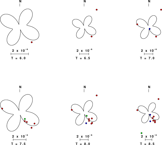
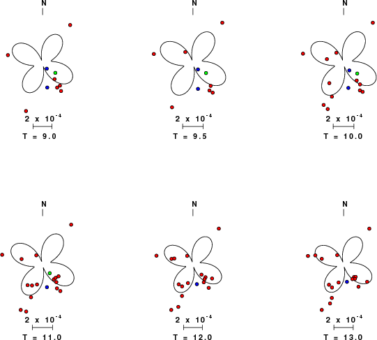
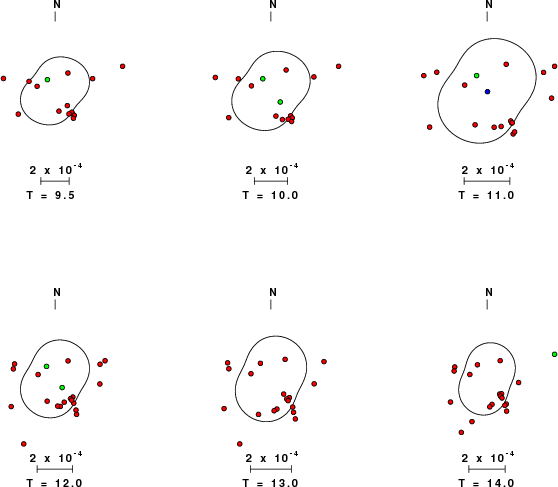
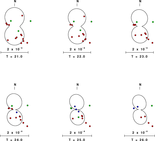
| Pressure-tension axis trends. Since the surface-wave spectra search does not distinguish between P and T axes and since there is a 180 ambiguity in strike, all possible P and T axes are plotted. First motion data and waveforms will be used to select the preferred mechanism. The purpose of this plot is to provide an idea of the possible range of solutions. The P and T-axes for all mechanisms with goodness of fit greater than 0.9 FITMAX (above) are plotted here. |

|
| Focal mechanism sensitivity at the preferred depth. The red color indicates a very good fit to the Love and Rayleigh wave radiation patterns. Each solution is plotted as a vector at a given value of strike and dip with the angle of the vector representing the rake angle, measured, with respect to the upward vertical (N) in the figure. Because of the symmetry of the spectral amplitude rediation patterns, only strikes from 0-180 degrees are sampled. |
Sta Az(deg)    Dist(km)
MSO	  326	  188
IMW	  142	  214
MOOW	  142	  236
HLID	  216	  254
LOHW	  142	  255
RLMT	   96	  261
SNOW	  146	  262
REDW	  149	  267
EGMT	   36	  360
BW06	  140	  381
HWUT	  169	  432
LAO	   72	  510
HAWA	  284	  551
WVOR	  238	  590
LON	  285	  729
PHWY	  126	  736
GNW	  290	  822
ISCO	  135	  846
NLWA	  288	  895
MVCO	  158	  974
TPNV	  199	  991
WUAZ	  174	 1105
GSC	  199	 1180
ISA	  207	 1193
AGMN	   70	 1310
OSI	  206	 1310
BAR	  195	 1459
Since the analysis of the surface-wave radiation patterns uses only spectral amplitudes and because the surfave-wave radiation patterns have a 180 degree symmetry, each surface-wave solution consists of four possible focal mechanisms corresponding to the interchange of the P- and T-axes and a roation of the mechanism by 180 degrees. To select one mechanism, P-wave first motion can be used. This was not possible in this case because all the P-wave first motions were emergent ( a feature of the P-wave wave takeoff angle, the station location and the mechanism). The other way to select among the mechanisms is to compute forward synthetics and compare the observed and predicted waveforms.
The velocity model used for the waveform fit is a modified Utah model .
The fits to the waveforms with the given mechanism are show below:

|
This figure shows the fit to the three components of motion (Z - vertical, R-radial and T - transverse). For each station and component, the observed traces is shown in red and the model predicted trace in blue. The traces represent filtered ground velocity in units of meters/sec (the peak value is printed adjacent to each trace; each pair of traces to plotted to the same scale to emphasize the difference in levels). Both synthetic and observed traces have been filtered using the SAC commands:
hp c 0.02 n 3
lp c 0.10 n 3
br c 0.12 0.25 n 4 p 2

|

|
Should the national backbone of the USGS Advanced National Seismic System (ANSS) be implemented with an interstation separation of 300 km, it is very likely that an earthquake such as this would have been recorded at distances on the order of 100-200 km. This means that the closest station would have information on source depth and mechanism that was lacking here.
Dr. Harley Benz, USGS, provided the USGS USNSN digital data. The digital data used in this study were provided by Natural Resources Canada through their AUTODRM site http://www.seismo.nrcan.gc.ca/nwfa/autodrm/autodrm_req_e.php, and IRIS using their BUD interface
The figures below show the observed spectral amplitudes (units of cm-sec) at each station and the
theoretical predictions as a function of period for the mechanism given above. The modified Utah model earth model
was used to define the Green's functions. For each station, the Love and Rayleigh wave spectrail amplitudes are plotted with the same scaling so that one can get a sense fo the effects of the effects of the focal mechanism and depth on the excitation of each.
 |
 |
 |
 |
 |
 |
 |
 |
 |
 |
 |
 |
 |
 |
 |
 |
 |
 |
 |
 |
 |
 |
 |
 |
 |
 |
 |
Here we tabulate the reasons for not using certain digital data sets
The following stations did not have a valid response files: