
2007/03/05 18:06:23 58.81N 134.44W 1 4.0 Alaska
USGS Felt map for this earthquake
USGS Felt reports page for Alaska
 SLU Moment Tensor Solution
 2007/03/05 18:06:23 58.81N 134.44W 1 4.0 Alaska

 Best Fitting Double Couple
    Mo = 6.53e+21 dyne-cm
    Mw = 3.81
    Z  = 1 km
     Plane   Strike  Dip  Rake
      NP1      221    55    93
      NP2       35    35    85
 Principal Axes:
   Axis    Value   Plunge  Azimuth
     T   6.53e+21     79     145
     N   0.00e+00      3      39
     P  -6.53e+21     10     309


 Moment Tensor: (dyne-cm)
    Component  Value
       Mxx    -2.32e+21
       Mxy     2.98e+21
       Mxz    -1.66e+21
       Myy    -3.80e+21
       Myz     1.56e+21
       Mzz     6.11e+21


                     --------------
                 ----------------------
              ---------------------------#
               -----------------##########-
           - P --------------#############---
          --   -----------#################---
         ---------------###################----
        --------------#####################-----
        ------------#######################-----
       ------------########################------
       -----------#########################------
       ----------###########   ###########-------
       ---------############ T ###########-------
        -------#############   ##########-------
        -------#########################--------
         -----#########################--------
          ----#######################---------
           ---#####################----------
             -###################----------
              ################------------
                 --####----------------
                     --------------


 Harvard Convention
 Moment Tensor:
      R          T          F
  6.11e+21  -1.66e+21  -1.56e+21
 -1.66e+21  -2.32e+21  -2.98e+21
 -1.56e+21  -2.98e+21  -3.80e+21


Details of the solution is found at

http://www.eas.slu.edu/eqc/eqc_mt/MECH.NA/20070305180622/index.html
|
      STK = 35
      DIP = 35
     RAKE = 85
       MW = 3.81
       HS = 1
The depth is not well determined. Both surface-wave and waveform inversion point to a more vertical dip-slip solution. The depth could be 8 km on the basis of the surface-wave spectral shapes.
The focal mechanism was determined using broadband seismic waveforms. The location of the event and the and stations used for the waveform inversion are shown in the next figure.
|
|
|
|
The program wvfgrd96 was used with good traces observed at short distance to determine the focal mechanism, depth and seismic moment. This technique requires a high quality signal and well determined velocity model for the Green functions. To the extent that these are the quality data, this type of mechanism should be preferred over the radiation pattern technique which requires the separate step of defining the pressure and tension quadrants and the correct strike.
The observed and predicted traces are filtered using the following gsac commands:
hp c 0.02 n 3
lp c 0.10 n 3
br c 0.16 0.3 n 4 p 2
The results of this grid search from 0.5 to 19 km depth are as follow:
           DEPTH  STK   DIP  RAKE   MW    FIT
WVFGRD96    0.5   215    55    90   3.77 0.5879
WVFGRD96    1.0    35    35    85   3.81 0.5882
WVFGRD96    2.0   210    65    80   3.91 0.5291
WVFGRD96    3.0    25    75    80   3.91 0.5005
WVFGRD96    4.0    20    80    75   3.88 0.5029
WVFGRD96    5.0    15    80    75   3.87 0.5027
WVFGRD96    6.0   200    85   -60   3.84 0.5075
WVFGRD96    7.0   195    80   -60   3.85 0.5137
WVFGRD96    8.0   185    70   -65   3.88 0.5158
WVFGRD96    9.0   185    70   -65   3.88 0.5191
WVFGRD96   10.0   190    75   -65   3.89 0.5169
WVFGRD96   11.0   185    70   -70   3.91 0.5169
WVFGRD96   12.0   180    65   -70   3.94 0.5159
WVFGRD96   13.0   175    60   -75   3.97 0.5131
WVFGRD96   14.0   170    60   -80   3.98 0.5092
WVFGRD96   15.0   170    60   -80   3.98 0.5035
WVFGRD96   16.0   165    55   -85   4.00 0.4959
WVFGRD96   17.0   165    55   -85   4.01 0.4874
WVFGRD96   18.0   345    55   -80   4.01 0.4791
WVFGRD96   19.0   345    55   -80   4.02 0.4725
The best solution is
WVFGRD96 1.0 35 35 85 3.81 0.5882
The mechanism correspond to the best fit is

|
|
|
The best fit as a function of depth is given in the following figure:

|
|
|
The comparison of the observed and predicted waveforms is given in the next figure. The red traces are the observed and the blue are the predicted. Each observed-predicted componnet is plotted to the same scale and peak amplitudes are indicated by the numbers to the left of each trace. The number in black at the rightr of each predicted traces it the time shift required for maximum correlation between the observed and predicted traces. This time shift is required because the synthetics are not computed at exactly the same distance as the observed and because the velocity model used in the predictions may not be perfect. A positive time shift indicates that the prediction is too fast and should be delayed to match the observed trace (shift to the right in this figure). A negative value indicates that the prediction is too slow. The bandpass filter used in the processing and for the display was
hp c 0.02 n 3
lp c 0.10 n 3
br c 0.16 0.3 n 4 p 2

|
|
|

|
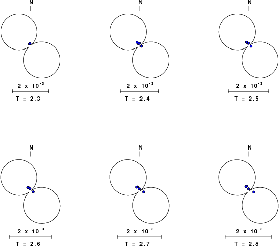
| Focal mechanism sensitivity at the preferred depth. The red color indicates a very good fit to thewavefroms. Each solution is plotted as a vector at a given value of strike and dip with the angle of the vector representing the rake angle, measured, with respect to the upward vertical (N) in the figure. |
The following figure shows the stations used in the grid search for the best focal mechanism to fit the surface-wave spectral amplitudes of the Love and Rayleigh waves.

|
|
|
The surface-wave determined focal mechanism is shown here.
  NODAL PLANES


  STK=     230.39
  DIP=      81.35
 RAKE=      95.04

             OR

  STK=      19.98
  DIP=      10.00
 RAKE=      59.97


DEPTH = 1.0 km

Mw = 4.17
Best Fit 0.8292 - P-T axis plot gives solutions with FIT greater than FIT90
 |
The P-wave first motion data for focal mechanism studies are as follow:
Sta Az(deg)    Dist(km)   First motion
SKAG      329   83 iP_C
WHY       355  205 iP_C
DLBC       97  267 iP_D
PNL       291  291 eP_X
CRAG      166  384 eP_X
DAWY      338  637 iP_D
Surface wave analysis was performed using codes from Computer Programs in Seismology, specifically the multiple filter analysis program do_mft and the surface-wave radiation pattern search program srfgrd96.
Digital data were collected, instrument response removed and traces converted
to Z, R an T components. Multiple filter analysis was applied to the Z and T traces to obtain the Rayleigh- and Love-wave spectral amplitudes, respectively.
These were input to the search program which examined all depths between 1 and 25 km
and all possible mechanisms.

|
|
|

|
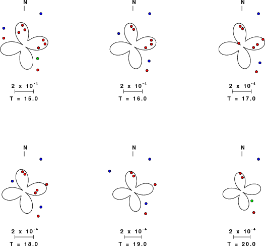
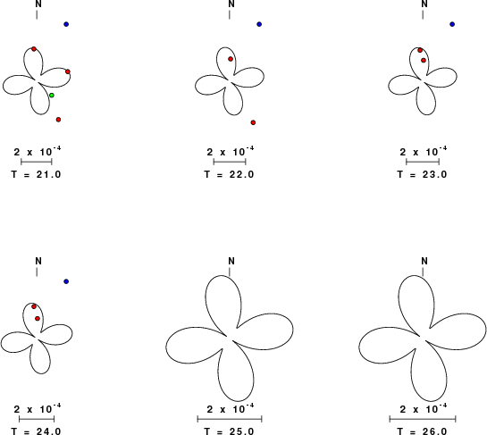
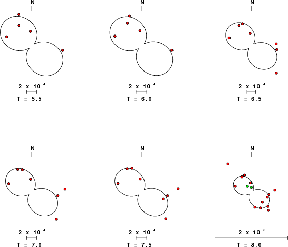
| Pressure-tension axis trends. Since the surface-wave spectra search does not distinguish between P and T axes and since there is a 180 ambiguity in strike, all possible P and T axes are plotted. First motion data and waveforms will be used to select the preferred mechanism. The purpose of this plot is to provide an idea of the possible range of solutions. The P and T-axes for all mechanisms with goodness of fit greater than 0.9 FITMAX (above) are plotted here. |

|
| Focal mechanism sensitivity at the preferred depth. The red color indicates a very good fit to the Love and Rayleigh wave radiation patterns. Each solution is plotted as a vector at a given value of strike and dip with the angle of the vector representing the rake angle, measured, with respect to the upward vertical (N) in the figure. Because of the symmetry of the spectral amplitude rediation patterns, only strikes from 0-180 degrees are sampled. |
The distribution of broadband stations with azimuth and distance is
Sta Az(deg)    Dist(km)
SKAG	  329	   83
WHY	  355	  205
DLBC	   98	  267
PNL	  291	  291
CRAG	  166	  384
RUBB	  150	  567
DAWY	  338	  637
FNBB	   84	  666
DOT	  321	  739
BMBC	  107	  807
BBB	  148	  844
BPAW	  311	 1049
INK	    2	 1058
COLD	  327	 1219
LLLB	  133	 1223
WSLR	  137	 1225
SLEB	  122	 1348
PNT	  131	 1436
FCC	   73	 2305
RES	   27	 2398
Since the analysis of the surface-wave radiation patterns uses only spectral amplitudes and because the surfave-wave radiation patterns have a 180 degree symmetry, each surface-wave solution consists of four possible focal mechanisms corresponding to the interchange of the P- and T-axes and a roation of the mechanism by 180 degrees. To select one mechanism, P-wave first motion can be used. This was not possible in this case because all the P-wave first motions were emergent ( a feature of the P-wave wave takeoff angle, the station location and the mechanism). The other way to select among the mechanisms is to compute forward synthetics and compare the observed and predicted waveforms.
The fits to the waveforms with the given mechanism are show below:

|
This figure shows the fit to the three components of motion (Z - vertical, R-radial and T - transverse). For each station and component, the observed traces is shown in red and the model predicted trace in blue. The traces represent filtered ground velocity in units of meters/sec (the peak value is printed adjacent to each trace; each pair of traces to plotted to the same scale to emphasize the difference in levels). Both synthetic and observed traces have been filtered using the SAC commands:
hp c 0.02 n 3
lp c 0.10 n 3
br c 0.16 0.3 n 4 p 2

|

|
Should the national backbone of the USGS Advanced National Seismic System (ANSS) be implemented with an interstation separation of 300 km, it is very likely that an earthquake such as this would have been recorded at distances on the order of 100-200 km. This means that the closest station would have information on source depth and mechanism that was lacking here.
Dr. Harley Benz, USGS, provided the USGS USNSN digital data. The digital data used in this study were provided by Natural Resources Canada through their AUTODRM site http://www.seismo.nrcan.gc.ca/nwfa/autodrm/autodrm_req_e.php, and IRIS using their BUD interface
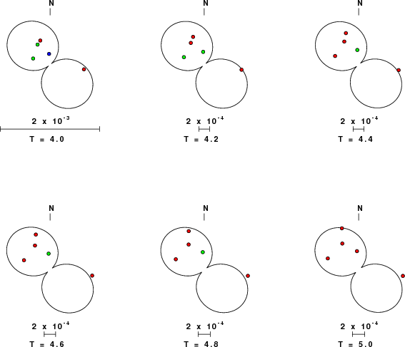
The figures below show the observed spectral amplitudes (units of cm-sec) at each station and the
theoretical predictions as a function of period for the mechanism given above. The CUS model earth model
was used to define the Green's functions. For each station, the Love and Rayleigh wave spectrail amplitudes are plotted with the same scaling so that one can get a sense fo the effects of the effects of the focal mechanism and depth on the excitation of each.
 |
 |
 |
 |
 |
 |
 |
 |
 |
 |
 |
 |
 |
 |
 |
 |
 |
 |
 |
 |
Here we tabulate the reasons for not using certain digital data sets
The following stations did not have a valid response files: