
2007/01/09 15:49:35 59.37N 136.87W 15 5.7 British Columbia, Canada
USGS Felt map for this earthquake
USGS Felt reports page for Canada
|
|
|
|
      STK = 275
      DIP = 60
     RAKE = 30
       MW = 5.59
       HS = 13
The surface-wave spectral amplitude solution is preferred since its Mw is closer to teleseismic estimates. The wavefrom inversion is similar except that the moment is about 0.18 units smaller.
The focal mechanism was determined using broadband seismic waveforms. The location of the event and the and stations used for the waveform inversion are shown in the next figure.
|
|
|
|
The program wvfgrd96 was used with good traces observed at short distance to determine the focal mechanism, depth and seismic moment. This technique requires a high quality signal and well determined velocity model for the Green functions. To the extent that these are the quality data, this type of mechanism should be preferred over the radiation pattern technique which requires the separate step of defining the pressure and tension quadrants and the correct strike.
The observed and predicted traces are filtered using the following gsac commands:
hp c 0.01 n 3
lp c 0.10 n 3
The results of this grid search from 0.5 to 19 km depth are as follow:
           DEPTH  STK   DIP  RAKE   MW    FIT
WVFGRD96    0.5   255    80   -35   5.25 0.5165
WVFGRD96    1.0   250    75   -40   5.27 0.5156
WVFGRD96    2.0   245    70   -55   5.36 0.4995
WVFGRD96    3.0   250    80   -65   5.42 0.4975
WVFGRD96    4.0   265    45     0   5.26 0.5321
WVFGRD96    5.0   265    45     5   5.27 0.5726
WVFGRD96    6.0   265    45     5   5.28 0.6080
WVFGRD96    7.0   265    50    10   5.30 0.6402
WVFGRD96    8.0   265    50    10   5.31 0.6675
WVFGRD96    9.0   265    50    10   5.32 0.6889
WVFGRD96   10.0   270    45    25   5.35 0.7074
WVFGRD96   11.0   270    45    25   5.36 0.7222
WVFGRD96   12.0   270    45    25   5.38 0.7333
WVFGRD96   13.0   270    45    25   5.39 0.7407
WVFGRD96   14.0   270    45    25   5.40 0.7448
WVFGRD96   15.0   270    45    25   5.41 0.7455
WVFGRD96   16.0   275    45    30   5.41 0.7434
WVFGRD96   17.0   275    45    30   5.42 0.7397
WVFGRD96   18.0   275    45    30   5.43 0.7335
WVFGRD96   19.0   275    45    30   5.44 0.7250
The best solution is
WVFGRD96 15.0 270 45 25 5.41 0.7455
The mechanism correspond to the best fit is

|
|
|
The best fit as a function of depth is given in the following figure:

|
|
|
The comparison of the observed and predicted waveforms is given in the next figure. The red traces are the observed and the blue are the predicted. Each observed-predicted componnet is plotted to the same scale and peak amplitudes are indicated by the numbers to the left of each trace. The number in black at the rightr of each predicted traces it the time shift required for maximum correlation between the observed and predicted traces. This time shift is required because the synthetics are not computed at exactly the same distance as the observed and because the velocity model used in the predictions may not be perfect. A positive time shift indicates that the prediction is too fast and should be delayed to match the observed trace (shift to the right in this figure). A negative value indicates that the prediction is too slow. The bandpass filter used in the processing and for the display was
hp c 0.01 n 3
lp c 0.10 n 3

|
|
|

|
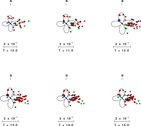
| Focal mechanism sensitivity at the preferred depth. The red color indicates a very good fit to thewavefroms. Each solution is plotted as a vector at a given value of strike and dip with the angle of the vector representing the rake angle, measured, with respect to the upward vertical (N) in the figure. |
The following figure shows the stations used in the grid search for the best focal mechanism to fit the surface-wave spectral amplitudes of the Love and Rayleigh waves.

|
|
|
The surface-wave determined focal mechanism is shown here.
  NODAL PLANES


  STK=     168.88
  DIP=      64.34
 RAKE=     146.31

             OR

  STK=     274.98
  DIP=      60.00
 RAKE=      30.00


DEPTH = 013.0 km

Mw = 5.59
Best Fit 0.8015 - P-T axis plot gives solutions with FIT greater than FIT90
 |
The P-wave first motion data for focal mechanism studies are as follow:
Sta Az(deg)    Dist(km)   First motion
SKAG       91   98 iP_D
PNL       280  134 iP_D
WHY        42  179 iP_D
WRAK      139  441 iP_C
EYAK      288  499 eP_X
CRAG      150  506 eP_X
Surface wave analysis was performed using codes from Computer Programs in Seismology, specifically the multiple filter analysis program do_mft and the surface-wave radiation pattern search program srfgrd96.
Digital data were collected, instrument response removed and traces converted
to Z, R an T components. Multiple filter analysis was applied to the Z and T traces to obtain the Rayleigh- and Love-wave spectral amplitudes, respectively.
These were input to the search program which examined all depths between 1 and 25 km
and all possible mechanisms.

|
|
|

|
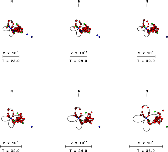
| Pressure-tension axis trends. Since the surface-wave spectra search does not distinguish between P and T axes and since there is a 180 ambiguity in strike, all possible P and T axes are plotted. First motion data and waveforms will be used to select the preferred mechanism. The purpose of this plot is to provide an idea of the possible range of solutions. The P and T-axes for all mechanisms with goodness of fit greater than 0.9 FITMAX (above) are plotted here. |

|
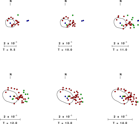
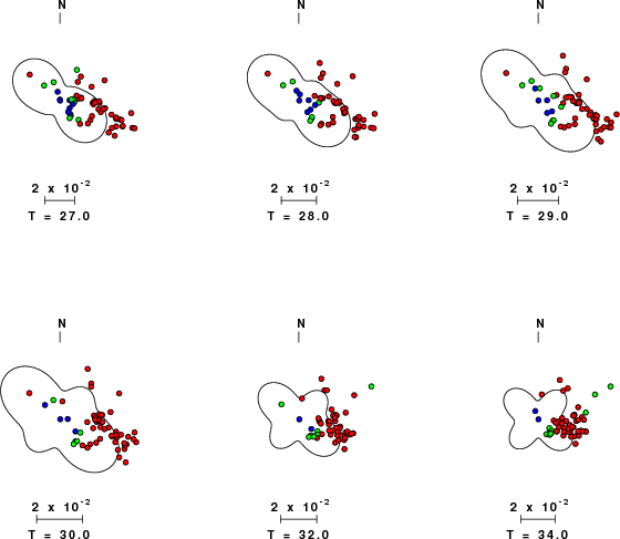
| Focal mechanism sensitivity at the preferred depth. The red color indicates a very good fit to the Love and Rayleigh wave radiation patterns. Each solution is plotted as a vector at a given value of strike and dip with the angle of the vector representing the rake angle, measured, with respect to the upward vertical (N) in the figure. Because of the symmetry of the spectral amplitude rediation patterns, only strikes from 0-180 degrees are sampled. |
The distribution of broadband stations with azimuth and distance is
Sta Az(deg)    Dist(km)
PNL	  280	  134
WRAK	  139	  441
CRAG	  150	  506
DAWY	  347	  541
PAX	  314	  596
EGAK	  342	  629
COLA	  322	  822
BPAW	  311	  895
PPLA	  302	  897
BMBC	  106	  952
BBB	  142	  986
INK	    8	 1000
COLD	  328	 1083
YKW3	   65	 1256
YKW1	   65	 1262
LLLB	  129	 1380
A05A	  134	 1516
B04A	  139	 1549
EDM	  105	 1600
TNA	  306	 1708
JCC	  151	 2268
RES	   29	 2405
FCC	   73	 2416
GASB	  149	 2427
LAO	  111	 2476
HOPS	  150	 2486
BW06	  122	 2643
HWUT	  127	 2656
ILON	   44	 2767
ULM	   93	 2786
RSSD	  113	 2803
EYMN	   93	 3196
MVCO	  128	 3210
PFO	  143	 3252
SDCO	  123	 3298
SNQN	   70	 3324
BAR	  144	 3342
CBKS	  114	 3487
FRB	   52	 3494
ANMO	  127	 3520
SCIA	  103	 3571
TUC	  136	 3595
KSU1	  110	 3626
GLMI	   92	 3820
WMOK	  118	 3907
SLM	  104	 4012
SFJD	   41	 4066
AAM	   94	 4074
SCHQ	   66	 4086
SADO	   87	 4135
SIUC	  104	 4147
BLO	  100	 4172
MIAR	  112	 4193
USIN	  102	 4211
UALR	  110	 4238
JCT	  122	 4260
WCI	  101	 4265
UTMT	  105	 4286
ALLY	   91	 4326
MPH	  107	 4336
WVT	  104	 4362
NATX	  116	 4393
LONY	   83	 4404
OXF	  107	 4419
FRNY	   82	 4444
PLAL	  106	 4450
NCB	   84	 4476
BINY	   87	 4518
SSPA	   90	 4537
ACCN	   84	 4554
LBNH	   82	 4584
KVTX	  122	 4634
BLA	   96	 4682
SDMD	   91	 4699
LTL	  112	 4709
BRNJ	   88	 4722
PAL	   87	 4733
CPNY	   87	 4748
CUNY	   87	 4760
CBN	   92	 4770
GOGA	  102	 4843
BRAL	  108	 4863
DRLN	   66	 4975
CNNC	   96	 4996
NHSC	   99	 5054
DWPF	  105	 5436
Since the analysis of the surface-wave radiation patterns uses only spectral amplitudes and because the surfave-wave radiation patterns have a 180 degree symmetry, each surface-wave solution consists of four possible focal mechanisms corresponding to the interchange of the P- and T-axes and a roation of the mechanism by 180 degrees. To select one mechanism, P-wave first motion can be used. This was not possible in this case because all the P-wave first motions were emergent ( a feature of the P-wave wave takeoff angle, the station location and the mechanism). The other way to select among the mechanisms is to compute forward synthetics and compare the observed and predicted waveforms.
The fits to the waveforms with the given mechanism are show below:

|
This figure shows the fit to the three components of motion (Z - vertical, R-radial and T - transverse). For each station and component, the observed traces is shown in red and the model predicted trace in blue. The traces represent filtered ground velocity in units of meters/sec (the peak value is printed adjacent to each trace; each pair of traces to plotted to the same scale to emphasize the difference in levels). Both synthetic and observed traces have been filtered using the SAC commands:
hp c 0.01 n 3
lp c 0.10 n 3

|

|
Should the national backbone of the USGS Advanced National Seismic System (ANSS) be implemented with an interstation separation of 300 km, it is very likely that an earthquake such as this would have been recorded at distances on the order of 100-200 km. This means that the closest station would have information on source depth and mechanism that was lacking here.
Dr. Harley Benz, USGS, provided the USGS USNSN digital data. The digital data used in this study were provided by Natural Resources Canada through their AUTODRM site http://www.seismo.nrcan.gc.ca/nwfa/autodrm/autodrm_req_e.php, and IRIS using their BUD interface
The figures below show the observed spectral amplitudes (units of cm-sec) at each station and the
theoretical predictions as a function of period for the mechanism given above. The CUS model earth model
was used to define the Green's functions. For each station, the Love and Rayleigh wave spectrail amplitudes are plotted with the same scaling so that one can get a sense fo the effects of the effects of the focal mechanism and depth on the excitation of each.
 |
 |
 |
 |
 |
 |
 |
 |
 |
 |
 |
 |
 |
 |
 |
 |
 |
 |
 |
 |
 |
 |
 |
 |
 |
 |
 |
 |
 |
 |
 |
 |
 |
 |
 |
 |
 |
 |
 |
 |
 |
 |
 |
 |
 |
 |
 |
 |
 |
 |
 |
 |
 |
 |
 |
 |
 |
 |
 |
 |
 |
 |
 |
 |
 |
 |
 |
 |
 |
 |
 |
 |
 |
 |
 |
 |
 |
 |
 |
 |
 |
 |
 |
 |
 |
 |
Here we tabulate the reasons for not using certain digital data sets
The following stations did not have a valid response files: