
2006/08/27 03:20:05  66.30N 142.16W  1.0*  4.4ML              280 km NW of Dawson,YT NRCAN
4.5 	2006/08/27 03:19:54	 66.952	-141.408	 2.3	NORTHERN ALASKA AIT (ANSS)
0.580      66.3319   -142.3828      10.0 20060827032003.349        1156648803.35
 ELOCATE
2006/08/27 03:20:05.88 66.302 -142.253 10.0 mag 4.5 (AEIC) prelim NEIC
2006/08/27 03:20:05 66.30N 142.25W 10 4.5 Alaska
USGS Felt map for this earthquake
USGS Felt reports page for Alaska
 SLU Moment Tensor Solution
 2006/08/27 03:20:05 66.30N 142.25W 10 4.5 Alaska

 Best Fitting Double Couple
    Mo = 3.76e+22 dyne-cm
    Mw = 4.35
    Z  = 20 km
     Plane   Strike  Dip  Rake
      NP1      319    76   -164
      NP2      225    75   -15
 Principal Axes:
   Axis    Value   Plunge  Azimuth
     T   3.76e+22      0      92
     N   0.00e+00     69       1
     P  -3.76e+22     21     182


 Moment Tensor: (dyne-cm)
    Component  Value
       Mxx    -3.26e+22
       Mxy    -2.43e+21
       Mxz     1.26e+22
       Myy     3.75e+22
       Myz     6.87e+20
       Mzz    -4.86e+21


                     --------------
                 ----------------------
              ----------------------------
             #####----------------------###
           ##########----------------########
          #############-----------############
         ################-------###############
        ###################--###################
        ###################--###################
       ##################-----###################
       #################--------###############
       ###############------------############# T
       #############---------------############
        ###########-----------------############
        ##########-------------------###########
         #######-----------------------########
          #####-------------------------######
           ###--------------------------#####
             #------------   ------------##
              ------------ P -------------
                 ---------   ----------
                     --------------


 Harvard Convention
 Moment Tensor:
      R          T          F
 -4.86e+21   1.26e+22  -6.87e+20
  1.26e+22  -3.26e+22   2.43e+21
 -6.87e+20   2.43e+21   3.75e+22


Details of the solution is found at

http://www.eas.slu.edu/eqc/eqc_mt/MECH.NA/20060827031954/index.html
|
The focal mechanism was determined using broadband seismic waveforms. The location of the event and the station distribution are given in Figure 1.
|
|
|
|
      STK = 225
      DIP = 75
     RAKE = -15
       MW = 4.35
       HS = 20
The waveform inversion is preferred although the depth may not be well controlled. The NEIS location is accepted. The surface-wave mechanism agrees with the waveform inversion but lacks depth control.
The program wvfgrd96 was used with good traces observed at short distance to determine the focal mechanism, depth and seismic moment. This technique requires a high quality signal and well determined velocity model for the Green functions. To the extent that these are the quality data, this type of mechanism should be preferred over the radiation pattern technique which requires the separate step of defining the pressure and tension quadrants and the correct strike.
The observed and predicted traces are filtered using the following gsac commands:
hp c 0.016 n 3
lp c 0.06 n 3
The results of this grid search from 0.5 to 19 km depth are as follow:
           DEPTH  STK   DIP  RAKE   MW    FIT
WVFGRD96    0.5   320    80   -35   4.22 0.5311
WVFGRD96    1.0   315    90   -20   4.19 0.5404
WVFGRD96    2.0   135    85    10   4.19 0.5531
WVFGRD96    3.0   135    85    10   4.20 0.5569
WVFGRD96    4.0   140    70    20   4.23 0.5576
WVFGRD96    5.0   315    75   -20   4.23 0.5597
WVFGRD96    6.0   310    75   -15   4.24 0.5624
WVFGRD96    7.0   310    70   -15   4.25 0.5652
WVFGRD96    8.0   310    70   -15   4.25 0.5685
WVFGRD96    9.0   315    75   -15   4.25 0.5714
WVFGRD96   10.0   310    70   -15   4.27 0.5730
WVFGRD96   11.0    50    75    15   4.26 0.5768
WVFGRD96   12.0   230    75    15   4.27 0.5811
WVFGRD96   13.0   230    75    15   4.28 0.5855
WVFGRD96   14.0   225    75   -15   4.29 0.5900
WVFGRD96   15.0   225    75   -15   4.30 0.5953
WVFGRD96   16.0   225    75   -15   4.31 0.5992
WVFGRD96   17.0   225    75   -15   4.32 0.6022
WVFGRD96   18.0   225    75   -15   4.33 0.6040
WVFGRD96   19.0   225    75   -15   4.34 0.6048
WVFGRD96   20.0   225    75   -15   4.35 0.6055
WVFGRD96   21.0   225    75   -15   4.36 0.6053
WVFGRD96   22.0   225    75   -15   4.36 0.6040
WVFGRD96   23.0   225    75   -15   4.37 0.6018
WVFGRD96   24.0   225    75   -15   4.38 0.5988
WVFGRD96   25.0   225    75   -15   4.39 0.5949
WVFGRD96   26.0   225    75   -15   4.40 0.5902
WVFGRD96   27.0   225    75   -15   4.40 0.5848
WVFGRD96   28.0   230    75   -15   4.41 0.5786
WVFGRD96   29.0   230    75   -15   4.41 0.5717
The best solution is
WVFGRD96 20.0 225 75 -15 4.35 0.6055
The mechanism correspond to the best fit is

|
|
|
The best fit as a function of depth is given in the following figure:

|
|
|
The comparison of the observed and predicted waveforms is given in the next figure. The red traces are the observed and the blue are the predicted. Each observed-predicted componnet is plotted to the same scale and peak amplitudes are indicated by the numbers to the left of each trace. The number in black at the rightr of each predicted traces it the time shift required for maximum correlation between the observed and predicted traces. This time shift is required because the synthetics are not computed at exactly the same distance as the observed and because the velocity model used in the predictions may not be perfect. A positive time shift indicates that the prediction is too fast and should be delayed to match the observed trace (shift to the right in this figure). A negative value indicates that the prediction is too slow. The bandpass filter used in the processing and for the display was
hp c 0.016 n 3
lp c 0.06 n 3

|
|
|

|
| Focal mechanism sensitivity at the preferred depth. The red color indicates a very good fit to thewavefroms. Each solution is plotted as a vector at a given value of strike and dip with the angle of the vector representing the rake angle, measured, with respect to the upward vertical (N) in the figure. |
  NODAL PLANES


  STK=     227.36
  DIP=      80.34
 RAKE=     -15.22

             OR

  STK=     319.97
  DIP=      75.00
 RAKE=    -169.99


DEPTH = 2.0 km

Mw = 4.15
Best Fit 0.7956 - P-T axis plot gives solutions with FIT greater than FIT90
 |
The P-wave first motion data for focal mechanism studies are as follow:
Sta Az(deg)    Dist(km)   First motion
DAWY      150  289 eP_X
COLD      290  359 iP_D
MCK       230  424 eP_X
INK        56  441 iP_C
BPAW      242  473 iP_+
TRF       233  493 eP_+
KTH       236  509 iP_C
CHUM      244  541 eP_X
WHY       152  772 eP_X
DLBC      143 1111 eP_X
Surface wave analysis was performed using codes from Computer Programs in Seismology, specifically the multiple filter analysis program do_mft and the surface-wave radiation pattern search program srfgrd96.

|
|
|
The velocity model used for the search is a CUS model .
Digital data were collected, instrument response removed and traces converted
to Z, R an T components. Multiple filter analysis was applied to the Z and T traces to obtain the Rayleigh- and Love-wave spectral amplitudes, respectively.
These were input to the search program which examined all depths between 1 and 25 km
and all possible mechanisms.

|
|
|

|
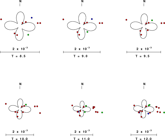
| Pressure-tension axis trends. Since the surface-wave spectra search does not distinguish between P and T axes and since there is a 180 ambiguity in strike, all possible P and T axes are plotted. First motion data and waveforms will be used to select the preferred mechanism. The purpose of this plot is to provide an idea of the possible range of solutions. The P and T-axes for all mechanisms with goodness of fit greater than 0.9 FITMAX (above) are plotted here. |

|
| Focal mechanism sensitivity at the preferred depth. The red color indicates a very good fit to the Love and Rayleigh wave radiation patterns. Each solution is plotted as a vector at a given value of strike and dip with the angle of the vector representing the rake angle, measured, with respect to the upward vertical (N) in the figure. Because of the symmetry of the spectral amplitude rediation patterns, only strikes from 0-180 degrees are sampled. |
Sta Az(deg)    Dist(km)
DAWY	  150	  283
COLA	  241	  304
COLD	  290	  365
MCK	  231	  426
INK	   55	  438
BPAW	  243	  477
TRF	  234	  496
KTH	  237	  512
PPLA	  236	  608
PMR	  216	  624
EYAK	  197	  665
RC01	  216	  689
FIB	  218	  693
WHY	  146	  728
PNL	  168	  754
SWD	  211	  780
SKAG	  152	  840
DLBC	  139	 1078
KDAK	  214	 1091
SIT	  157	 1093
OHAK	  215	 1165
FNBB	  121	 1281
COWN	   80	 1415
GLWN	   81	 1518
MLON	   85	 1525
RES	   41	 1928
EDM	  119	 2149
SRLN	   57	 2445
ILON	   55	 2466
FFC	  101	 2501
WALA	  126	 2517
FCC	   86	 2547
HAWA	  138	 2594
EGMT	  121	 2772
BMO	  136	 2820
BOZ	  126	 2933
HLID	  132	 3045
ULM	  102	 3149
BW06	  126	 3294
ELK	  136	 3307
EYMN	  100	 3546
Since the analysis of the surface-wave radiation patterns uses only spectral amplitudes and because the surfave-wave radiation patterns have a 180 degree symmetry, each surface-wave solution consists of four possible focal mechanisms corresponding to the interchange of the P- and T-axes and a roation of the mechanism by 180 degrees. To select one mechanism, P-wave first motion can be used. This was not possible in this case because all the P-wave first motions were emergent ( a feature of the P-wave wave takeoff angle, the station location and the mechanism). The other way to select among the mechanisms is to compute forward synthetics and compare the observed and predicted waveforms.
The velocity model used for the waveform fit is a modified Utah model .
The fits to the waveforms with the given mechanism are show below:

|
This figure shows the fit to the three components of motion (Z - vertical, R-radial and T - transverse). For each station and component, the observed traces is shown in red and the model predicted trace in blue. The traces represent filtered ground velocity in units of meters/sec (the peak value is printed adjacent to each trace; each pair of traces to plotted to the same scale to emphasize the difference in levels). Both synthetic and observed traces have been filtered using the SAC commands:
hp c 0.016 n 3
lp c 0.06 n 3

|

|
Should the national backbone of the USGS Advanced National Seismic System (ANSS) be implemented with an interstation separation of 300 km, it is very likely that an earthquake such as this would have been recorded at distances on the order of 100-200 km. This means that the closest station would have information on source depth and mechanism that was lacking here.
Dr. Harley Benz, USGS, provided the USGS USNSN digital data. The digital data used in this study were provided by Natural Resources Canada through their AUTODRM site http://www.seismo.nrcan.gc.ca/nwfa/autodrm/autodrm_req_e.php, and IRIS using their BUD interface
The figures below show the observed spectral amplitudes (units of cm-sec) at each station and the
theoretical predictions as a function of period for the mechanism given above. The modified Utah model earth model
was used to define the Green's functions. For each station, the Love and Rayleigh wave spectrail amplitudes are plotted with the same scaling so that one can get a sense fo the effects of the effects of the focal mechanism and depth on the excitation of each.
 |
 |
 |
 |
 |
 |
 |
 |
 |
 |
 |
 |
 |
 |
 |
 |
 |
 |
 |
 |
 |
 |
 |
 |
 |
 |
 |
 |
 |
 |
 |
 |
 |
 |
 |
 |
 |
 |
 |
 |
 |
Here we tabulate the reasons for not using certain digital data sets
The following stations did not have a valid response files: