
2006/03/05 10:42:16 64.93N 129.26W 10 5.6 Canada
USGS Felt map for this earthquake
USGS Felt reports page for northwestern, Canada
 SLU Moment Tensor Solution
 2006/03/05 10:42:16 64.93N 129.26W 10 5.6 Canada

 Best Fitting Double Couple
    Mo = 1.51e+24 dyne-cm
    Mw = 5.42
    Z  = 2 km
     Plane   Strike  Dip  Rake
      NP1      117    45    95
      NP2      290    45    85
 Principal Axes:
   Axis    Value   Plunge  Azimuth
     T   1.51e+24     86     112
     N   0.00e+00      4     294
     P  -1.51e+24      0     204


 Moment Tensor: (dyne-cm)
    Component  Value
       Mxx    -1.27e+24
       Mxy    -5.56e+23
       Mxz    -3.19e+22
       Myy    -2.36e+23
       Myz     8.77e+22
       Mzz     1.51e+24


                     --------------
                 ----------------------
              ----------------------------
             ------------------------------
           --------#######-------------------
          ---####################-------------
         ############################----------
        --#############################---------
        --###############################-------
       ----################################------
       -----#################   #############----
       ------################ T ##############---
       -------###############   ##############---
        --------###############################-
        ----------#############################-
         -----------###########################
          -------------######################-
           -----------------#############----
             ------------------------------
              ----------------------------
                 ---   ----------------
                     P ------------


 Harvard Convention
 Moment Tensor:
      R          T          F
  1.51e+24  -3.19e+22  -8.77e+22
 -3.19e+22  -1.27e+24   5.56e+23
 -8.77e+22   5.56e+23  -2.36e+23


Details of the solution is found at

http://www.eas.slu.edu/eqc/eqc_mt/NEW/20060305104216/index.html
|
March 5, 2006, NORTHWEST TERRITORIES, CANADA, MW=5.5

Natasha Maternovskaya

CENTROID, MOMENT TENSOR SOLUTION
HARVARD EVENT-FILE NAME C030506B
DATA USED: GSN
L.P. BODY WAVES: 61S,123C, T= 40
SURFACE WAVES:   81S,181C, T= 50
CENTROID LOCATION:
ORIGIN TIME       10:42:19.6 0.1
LAT 65.05N 0.01;LON 129.19W 0.03
DEP  12.0 FIX;HALF-DURATION  1.3
MOMENT TENSOR; SCALE 10**24 D-CM
  MRR= 1.88 0.03; MTT=-1.68 0.02
  MPP=-0.21 0.02; MRT= 0.13 0.07
  MRP=-0.13 0.07; MTP= 0.70 0.02
 PRINCIPAL AXES:
 1.(T) VAL=  1.89;PLG=87;AZM= 64
 2.(N)       0.07;     2;    292
 3.(P)      -1.96;     2;    202
BEST DOUBLE COUPLE:M0=1.9*10**24
 NP1:STRIKE=289;DIP=43;SLIP=  87
 NP2:STRIKE=114;DIP=48;SLIP=  93

            -----------
        -------------------
      -----------------------
    ---------------------------
   ---################----------
  -######################--------
  -#########################-----
 --##############   ##########----
 ---############# T ###########---
 ----############   ############--
 ------##########################-
  -------########################
  ----------#####################
   ------------###############--
    ---------------------------
      -----------------------
        --   --------------
           P ----------
|
The focal mechanism was determined using broadband seismic waveforms. The location of the event and the station distribution are given in Figure 1.
|
|
|
|
      STK = 290
      DIP = 45
     RAKE = 85
       MW = 5.42
       HS = 2
The waveform solution is preferred. It agrees with the surface-wave solution.
The program wvfgrd96 was used with good traces observed at short distance to determine the focal mechanism, depth and seismic moment. This technique requires a high quality signal and well determined velocity model for the Green functions. To the extent that these are the quality data, this type of mechanism should be preferred over the radiation pattern technique which requires the separate step of defining the pressure and tension quadrants and the correct strike.
The observed and predicted traces are filtered using the following gsac commands:
hp c 0.016 3
lp c 0.06 3
The results of this grid search from 0.5 to 19 km depth are as follow:
           DEPTH  STK   DIP  RAKE   MW    FIT
WVFGRD96    0.5   275    45    60   5.33 0.5207
WVFGRD96    1.0   280    50    70   5.35 0.5400
WVFGRD96    2.0   290    45    85   5.42 0.5721
WVFGRD96    3.0   295    45    90   5.46 0.5479
WVFGRD96    4.0   285    30    80   5.49 0.4986
WVFGRD96    5.0   280    30    75   5.48 0.4778
WVFGRD96    6.0   280    30    75   5.47 0.4631
WVFGRD96    7.0   290    25    85   5.45 0.4529
WVFGRD96    8.0    55    50   -25   5.38 0.4630
WVFGRD96    9.0    55    55   -25   5.39 0.4754
WVFGRD96   10.0   100    25    75   5.45 0.4775
WVFGRD96   11.0    50    50   -35   5.42 0.4896
WVFGRD96   12.0    50    50   -35   5.43 0.5030
WVFGRD96   13.0    50    50   -35   5.43 0.5142
WVFGRD96   14.0    55    55   -35   5.44 0.5236
WVFGRD96   15.0    55    55   -35   5.44 0.5314
WVFGRD96   16.0    55    55   -35   5.45 0.5376
WVFGRD96   17.0    55    55   -30   5.45 0.5426
WVFGRD96   18.0    55    55   -30   5.46 0.5464
WVFGRD96   19.0    50    55   -35   5.47 0.5494
WVFGRD96   20.0    50    55   -35   5.49 0.5430
WVFGRD96   21.0    50    55   -35   5.49 0.5425
WVFGRD96   22.0    55    55   -30   5.49 0.5413
WVFGRD96   23.0    55    55   -30   5.50 0.5391
WVFGRD96   24.0    85    45    50   5.51 0.5392
WVFGRD96   25.0    85    45    50   5.51 0.5386
WVFGRD96   26.0    75    50    35   5.52 0.5370
WVFGRD96   27.0    75    50    35   5.52 0.5352
WVFGRD96   28.0    75    50    35   5.53 0.5326
WVFGRD96   29.0    75    50    35   5.54 0.5292
The best solution is
WVFGRD96 2.0 290 45 85 5.42 0.5721
The mechanism correspond to the best fit is

|
|
|
The best fit as a function of depth is given in the following figure:

|
|
|
The comparison of the observed and predicted waveforms is given in the next figure. The red traces are the observed and the blue are the predicted. Each observed-predicted componnet is plotted to the same scale and peak amplitudes are indicated by the numbers to the left of each trace. The number in black at the rightr of each predicted traces it the time shift required for maximum correlation between the observed and predicted traces. This time shift is required because the synthetics are not computed at exactly the same distance as the observed and because the velocity model used in the predictions may not be perfect. A positive time shift indicates that the prediction is too fast and should be delayed to match the observed trace (shift to the right in this figure). A negative value indicates that the prediction is too slow. The bandpass filter used in the processing and for the display was
hp c 0.016 3
lp c 0.06 3

|
|
|

|
| Focal mechanism sensitivity at the preferred depth. The red color indicates a very good fit to thewavefroms. Each solution is plotted as a vector at a given value of strike and dip with the angle of the vector representing the rake angle, measured, with respect to the upward vertical (N) in the figure. |
  NODAL PLANES


  STK=     302.15
  DIP=      55.61
 RAKE=      96.94

             OR

  STK=     109.99
  DIP=      35.00
 RAKE=      79.99


DEPTH = 2.0 km

Mw = 5.46
Best Fit 0.8362 - P-T axis plot gives solutions with FIT greater than FIT90
 |
The P-wave first motion data for focal mechanism studies are as follow:
Sta Az(deg)    Dist(km)   First motion
INK       335  421 eP_-
DAWY      263  497 eP_-
WHY       214  557 eP_X
GALN       94  580 eP_X
SKAG      210  688 eP_+
DOT       265  731 eP_-
FNBB      151  750 eP_X
BESE      205  768 eP_-
PNL       226  788 eP_-
DCPH      220  802 eP_X
PAX       262  823 eP_X
HARP      258  835 eP_X
LUPN       76  841 eP_-
BMR       247  894 eP_X
MLON       88  936 eP_X
SIT       203  938 -12345
MCK       271  959 -12345
EYAK      247  972 eP_X
COLD      295  978 eP_D
TRF       270 1032 eP_+
BPAW      275 1044 eP_+
KTH       272 1059 eP_+
PMR       259 1062 -12345
Surface wave analysis was performed using codes from Computer Programs in Seismology, specifically the multiple filter analysis program do_mft and the surface-wave radiation pattern search program srfgrd96.
Digital data were collected, instrument response removed and traces converted
to Z, R an T components. Multiple filter analysis was applied to the Z and T traces to obtain the Rayleigh- and Love-wave spectral amplitudes, respectively.
These were input to the search program which examined all depths between 1 and 25 km
and all possible mechanisms.

|
|
|

|
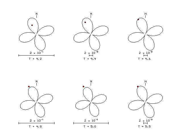
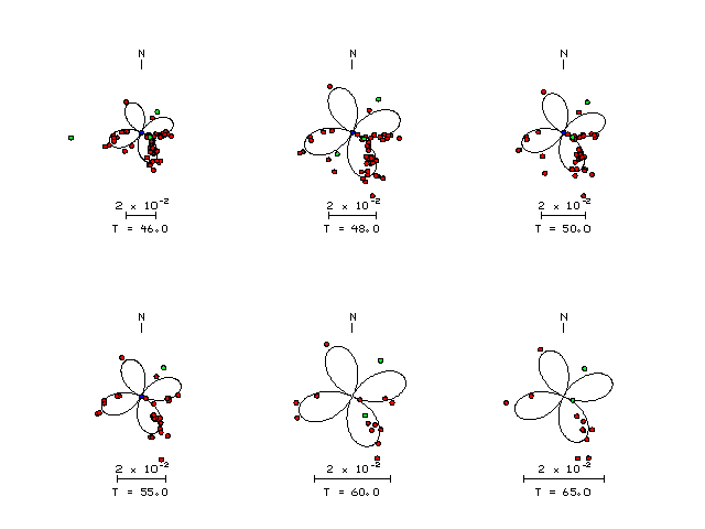
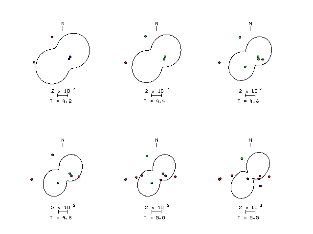
| Pressure-tension axis trends. Since the surface-wave spectra search does not distinguish between P and T axes and since there is a 180 ambiguity in strike, all possible P and T axes are plotted. First motion data and waveforms will be used to select the preferred mechanism. The purpose of this plot is to provide an idea of the possible range of solutions. The P and T-axes for all mechanisms with goodness of fit greater than 0.9 FITMAX (above) are plotted here. |

|
| Focal mechanism sensitivity at the preferred depth. The red color indicates a very good fit to the Love and Rayleigh wave radiation patterns. Each solution is plotted as a vector at a given value of strike and dip with the angle of the vector representing the rake angle, measured, with respect to the upward vertical (N) in the figure. Because of the symmetry of the spectral amplitude rediation patterns, only strikes from 0-180 degrees are sampled. |
The distribution of broadband stations with azimuth and distance is
Sta Az(deg)    Dist(km)
INK	  335	  421
DAWY	  263	  497
WHY	  214	  557
GALN	   94	  580
SKAG	  210	  688
DOT	  265	  731
FNBB	  151	  750
BESE	  205	  768
YKW2	  104	  776
YKW1	  104	  779
PNL	  226	  788
DCPH	  220	  802
PAX	  262	  823
HARP	  258	  835
LUPN	   76	  841
BMR	  247	  894
DIV	  251	  935
MLON	   88	  936
SIT	  203	  938
MCK	  271	  959
EYAK	  247	  972
COLD	  294	  978
TRF	  270	 1032
BPAW	  275	 1044
KTH	  272	 1059
PMR	  259	 1062
BMBC	  155	 1065
CRAG	  193	 1077
CHUM	  274	 1114
RC01	  257	 1118
FIB	  258	 1134
PPLA	  269	 1143
EDM	  138	 1584
LLLB	  161	 1654
RES	   35	 1674
TNA	  290	 1783
PNT	  157	 1832
OFR	  169	 1918
OCWA	  168	 1940
FCC	   94	 1948
NEW	  153	 1995
SDPT	  253	 2009
D03A	  168	 2014
E04A	  166	 2083
HAWA	  159	 2150
EGMT	  139	 2216
MSO	  148	 2221
HEBO	  169	 2224
G04A	  166	 2238
H02A	  169	 2281
TOLO	  169	 2288
COR	  168	 2298
AKUT	  257	 2346
DGMT	  129	 2361
I03A	  168	 2365
WIFE	  165	 2372
TAKO	  170	 2383
UNV	  257	 2403
BOZ	  145	 2405
I06A	  162	 2406
LAO	  134	 2465
K01A	  171	 2484
HUMO	  168	 2519
K06A	  163	 2531
ULM	  114	 2532
HLID	  152	 2556
NIKO	  258	 2585
WVOR	  160	 2595
YBH	  168	 2618
M04C	  166	 2622
MOD	  163	 2628
M02C	  168	 2654
JCC	  170	 2707
AHID	  146	 2721
HATC	  166	 2733
BILL	  306	 2756
BW06	  144	 2763
HWUT	  148	 2832
BMN	  158	 2837
ORV	  166	 2871
SUTB	  167	 2904
HOPS	  169	 2917
DUG	  151	 2952
TPH	  159	 3093
ISCO	  140	 3187
KAPO	  100	 3206
BAK	  163	 3364
SUMG	   36	 3400
GSC	  160	 3403
SDCO	  141	 3404
CBKS	  132	 3482
WUAZ	  151	 3486
NEE	  156	 3494
VLDQ	   97	 3537
KSU1	  128	 3566
Y22C	  145	 3751
AAM	  109	 3795
TUC	  152	 3844
SLM	  120	 3863
CCM	  122	 3879
FVM	  121	 3919
WMOK	  134	 3932
BLO	  115	 3966
SIUC	  120	 3995
LONY	   97	 4001
ACSO	  110	 4020
USIN	  118	 4035
MNTX	  144	 4045
NCB	   98	 4076
PVMO	  121	 4103
MIAR	  127	 4138
UTMT	  120	 4144
ACCN	   98	 4155
BINY	  101	 4155
LBNH	   95	 4160
UALR	  126	 4162
WRPS	  104	 4198
WVT	  119	 4208
MCWV	  107	 4214
MPH	  122	 4222
OXF	  122	 4304
HRV	   96	 4334
JCT	  138	 4340
MVL	  103	 4342
LTX	  143	 4344
TZTN	  114	 4349
BRNJ	  101	 4361
PAL	  100	 4362
SDMD	  104	 4375
FOR	  100	 4376
CPNY	  100	 4379
NATX	  130	 4382
BLA	  110	 4422
CBN	  106	 4464
HKT	  133	 4526
LRAL	  120	 4549
LTL	  126	 4652
NHSC	  113	 4831
DWPF	  117	 5272
Since the analysis of the surface-wave radiation patterns uses only spectral amplitudes and because the surfave-wave radiation patterns have a 180 degree symmetry, each surface-wave solution consists of four possible focal mechanisms corresponding to the interchange of the P- and T-axes and a roation of the mechanism by 180 degrees. To select one mechanism, P-wave first motion can be used. This was not possible in this case because all the P-wave first motions were emergent ( a feature of the P-wave wave takeoff angle, the station location and the mechanism). The other way to select among the mechanisms is to compute forward synthetics and compare the observed and predicted waveforms.
The fits to the waveforms with the given mechanism are show below:

|
This figure shows the fit to the three components of motion (Z - vertical, R-radial and T - transverse). For each station and component, the observed traces is shown in red and the model predicted trace in blue. The traces represent filtered ground velocity in units of meters/sec (the peak value is printed adjacent to each trace; each pair of traces to plotted to the same scale to emphasize the difference in levels). Both synthetic and observed traces have been filtered using the SAC commands:
hp c 0.016 3
lp c 0.06 3

|

|
Should the national backbone of the USGS Advanced National Seismic System (ANSS) be implemented with an interstation separation of 300 km, it is very likely that an earthquake such as this would have been recorded at distances on the order of 100-200 km. This means that the closest station would have information on source depth and mechanism that was lacking here.
Dr. Harley Benz, USGS, provided the USGS USNSN digital data.
The figures below show the observed spectral amplitudes (units of cm-sec) at each station and the
theoretical predictions as a function of period for the mechanism given above. The modified Utah model earth model
was used to define the Green's functions. For each station, the Love and Rayleigh wave spectrail amplitudes are plotted with the same scaling so that one can get a sense fo the effects of the effects of the focal mechanism and depth on the excitation of each.
 |
 |
 |
 |
 |
 |
 |
 |
 |
 |
 |
 |
 |
 |
 |
 |
 |
 |
 |
 |
 |
 |
 |
 |
 |
 |
 |
 |
 |
 |
 |
 |
 |
 |
 |
 |
 |
 |
 |
 |
 |
 |
 |
 |
 |
 |
 |
 |
 |
 |
 |
 |
 |
 |
 |
 |
 |
 |
 |
 |
 |
 |
 |
 |
 |
 |
 |
 |
 |
 |
 |
 |
 |
 |
 |
 |
 |
 |
 |
 |
 |
 |
 |
 |
 |
 |
 |
 |
 |
 |
 |
 |
 |
 |
 |
 |
 |
 |
 |
 |
 |
 |
 |
 |
 |
 |
 |
 |
 |
 |
 |
 |
 |
 |
 |
 |
 |
 |
 |
 |
 |
 |
 |
 |
 |
 |
 |
 |
 |
 |
 |
 |
 |
 |
 |
 |
 |
 |
 |
Here we tabulate the reasons for not using certain digital data sets
The following stations did not have a valid response files: