
2005/08/10 22:08:17 36.95N 104.86W 5. 4.9 New Mexico
USGS Felt map for this earthquake
USGS Felt reports page for Intermountain Western US
 SLU Moment Tensor Solution
 2005/08/10 22:08:17 36.95N 104.86W   5. 4.9 New Mexico

 Best Fitting Double Couple
    Mo = 2.34e+23 dyne-cm
    Mw = 4.88
    Z  = 4 km
     Plane   Strike  Dip  Rake
      NP1        5    53   -74
      NP2      160    40   -110
 Principal Axes:
   Axis    Value   Plunge  Azimuth
     T   2.34e+23      7      84
     N   0.00e+00     13     176
     P  -2.34e+23     76     327


 Moment Tensor: (dyne-cm)
    Component  Value
       Mxx    -7.75e+21
       Mxy     3.02e+22
       Mxz    -4.46e+22
       Myy     2.25e+23
       Myz     5.70e+22
       Mzz    -2.17e+23


                     ----------####
                 ##--------------######
              ####----------------########
             ####------------------########
           #####--------------------#########
          #####---------------------##########
         ######----------------------##########
        #######----------------------###########
        #######----------   ---------#########
       ########---------- P ---------######### T
       ########----------   ---------#########
       ########----------------------############
       #########---------------------############
        ########---------------------###########
        #########-------------------############
         #########------------------###########
          #########----------------###########
           ##########-------------###########
             ##########----------##########
              ###########-------##########
                 ###########--#########
                     #######------#


 Harvard Convention
 Moment Tensor:
      R          T          F
 -2.17e+23  -4.46e+22  -5.70e+22
 -4.46e+22  -7.75e+21  -3.02e+22
 -5.70e+22  -3.02e+22   2.25e+23


Details of the solution is found at

http://www.eas.slu.edu/eqc/eqc_mt/NEW/20050810220817/index.html
|
August 10, 2005, NEW MEXICO, MW=5.0

Meredith Nettles
Goran Ekstrom

CENTROID, MOMENT TENSOR SOLUTION
HARVARD EVENT-FILE NAME C081005B
DATA USED: GSN
L.P. BODY WAVES: 37S, 48C, T= 40
SURFACE WAVES:   53S, 99C, T= 50
CENTROID LOCATION:
ORIGIN TIME       22:08:23.6 0.2
LAT 36.90N 0.02;LON 104.80W 0.01
DEP  12.0 FIX;HALF-DURATION  0.8
MOMENT TENSOR; SCALE 10**23 D-CM
  MRR=-3.28 0.09; MTT=-0.37 0.09
  MPP= 3.65 0.08; MRT=-0.53 0.27
  MRP= 0.11 0.24; MTP=-0.65 0.08
 PRINCIPAL AXES:
 1.(T) VAL=  3.76;PLG= 2;AZM=261
 2.(N)      -0.38;    10;    171
 3.(P)      -3.37;    80;    360
BEST DOUBLE COUPLE:M0=3.6*10**23
 NP1:STRIKE=  1;DIP=44;SLIP= -76
 NP2:STRIKE=161;DIP=47;SLIP=-103

            -------####
        ###----------######
      ####-------------######
    #####---------------#######
   ######----------------#######
  ######------------------#######
  ######--------   -------#######
 #######-------- P -------########
 ########-------   --------#######
   ######------------------#######
 T ######-----------------########
   #######----------------#######
  #########---------------#######
   #########-------------#######
    ##########----------#######
      #########--------######
        ##########---######
            #######----
|
The focal mechanism was determined using broadband seismic waveforms. The location of the event and the station distribution are given in Figure 1.
|
|
|
|
      STK = 160
      DIP = 40
     RAKE = -110
       MW = 4.88
       HS = 4
The surface-wave is preferred because of the greater quantity of data and sensitivity to source depth. The waveform inversion had enough data after selective editing of traces. In this case the surface-wave analysis provided a quality control on the waveform data. SDCO horizontals could not be used because of questions of instrument polarity. The waveform fit was based on the use of a lower than normal lowpass filter because of neither set of Greens functions are appropriate to this region.
The program wvfgrd96 was used with good traces observed at short distance to determine the focal mechanism, depth and seismic moment. This technique requires a high quality signal and well determined velocity model for the Green functions. To the extent that these are the quality data, this type of mechanism should be preferred over the radiation pattern technique which requires the separate step of defining the pressure and tension quadrants and the correct strike.
The observed and predicted traces are filtered using the following gsac commands:
hp c 0.014 3
lp c 0.05 3
The results of this grid search from 0.5 to 19 km depth are as follow:
           DEPTH  STK   DIP  RAKE   MW    FIT
WVFGRD96    0.5    25    50   -60   4.62 0.4585
WVFGRD96    1.0    20    45   -65   4.65 0.4832
WVFGRD96    2.0    20    45   -65   4.71 0.5397
WVFGRD96    3.0    10    45   -80   4.74 0.5545
WVFGRD96    4.0    10    50   -75   4.77 0.5505
WVFGRD96    5.0   360    50   -85   4.80 0.5556
WVFGRD96    6.0   360    50   -85   4.81 0.5298
WVFGRD96    7.0   360    50   -85   4.81 0.4895
WVFGRD96    8.0   180    35   -90   4.83 0.4914
WVFGRD96    9.0   110    70    30   4.70 0.4650
WVFGRD96   10.0   110    70    30   4.70 0.4524
WVFGRD96   11.0   225    65   -35   4.74 0.4452
WVFGRD96   12.0   230    70   -30   4.74 0.4481
WVFGRD96   13.0   225    65   -30   4.74 0.4546
WVFGRD96   14.0   225    65   -30   4.74 0.4602
WVFGRD96   15.0   225    70   -30   4.74 0.4679
WVFGRD96   16.0   225    70   -30   4.74 0.4755
WVFGRD96   17.0   225    70   -25   4.75 0.4796
WVFGRD96   18.0   225    70   -25   4.76 0.4859
WVFGRD96   19.0   225    70   -25   4.76 0.4869
The best solution is
WVFGRD96 5.0 360 50 -85 4.80 0.5556
The mechanism correspond to the best fit is

|
|
|
The best fit as a function of depth is given in the following figure:

|
|
|
The comparison of the observed and predicted waveforms is given in the next figure. The red traces are the observed and the blue are the predicted. Each observed-predicted componnet is plotted to the same scale and peak amplitudes are indicated by the numbers to the left of each trace. The number in black at the rightr of each predicted traces it the time shift required for maximum correlation between the observed and predicted traces. This time shift is required because the synthetics are not computed at exactly the same distance as the observed and because the velocity model used in the predictions may not be perfect. A positive time shift indicates that the prediction is too fast and should be delayed to match the observed trace (shift to the right in this figure). A negative value indicates that the prediction is too slow. The bandpass filter used in the processing and for the display was
hp c 0.014 3
lp c 0.05 3

|
|
|

|
| Focal mechanism sensitivity at the preferred depth. The red color indicates a very good fit to thewavefroms. Each solution is plotted as a vector at a given value of strike and dip with the angle of the vector representing the rake angle, measured, with respect to the upward vertical (N) in the figure. |
  NODAL PLANES


  STK=       5.40
  DIP=      52.84
 RAKE=     -73.99

             OR

  STK=     160.00
  DIP=      40.00
 RAKE=    -109.99


DEPTH = 4.0 km

Mw = 4.88
Best Fit 0.8921 - P-T axis plot gives solutions with FIT greater than FIT90
 |
The P-wave first motion data for focal mechanism studies are as follow:
Sta Az(deg)    Dist(km)   First motion
ANMO      213  265 eP_-
ISCO      348  323 iP_D
Y22C      211  370 eP_X
CBKS       64  496 iP_C
Surface wave analysis was performed using codes from Computer Programs in Seismology, specifically the multiple filter analysis program do_mft and the surface-wave radiation pattern search program srfgrd96.
The velocity model used for the search is a modified Utah model .
Digital data were collected, instrument response removed and traces converted
to Z, R an T components. Multiple filter analysis was applied to the Z and T traces to obtain the Rayleigh- and Love-wave spectral amplitudes, respectively.
These were input to the search program which examined all depths between 1 and 25 km
and all possible mechanisms.

|
|
|

|
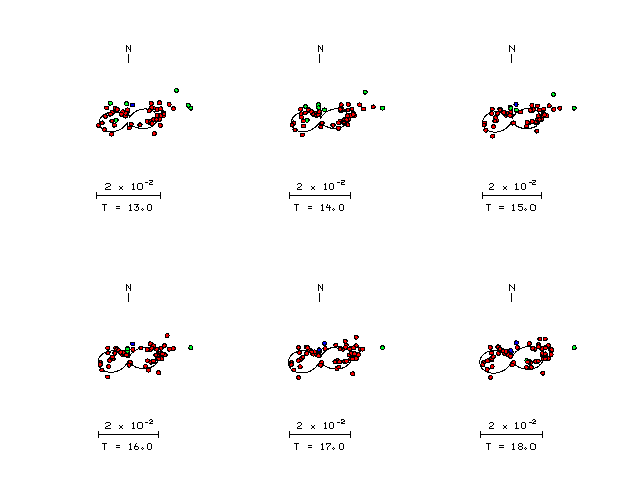
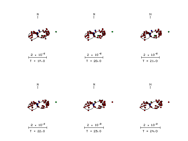
| Pressure-tension axis trends. Since the surface-wave spectra search does not distinguish between P and T axes and since there is a 180 ambiguity in strike, all possible P and T axes are plotted. First motion data and waveforms will be used to select the preferred mechanism. The purpose of this plot is to provide an idea of the possible range of solutions. The P and T-axes for all mechanisms with goodness of fit greater than 0.9 FITMAX (above) are plotted here. |

|
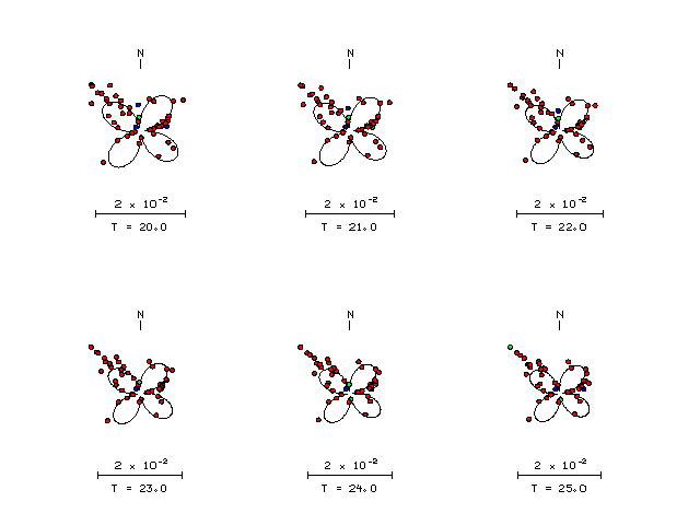
| Focal mechanism sensitivity at the preferred depth. The red color indicates a very good fit to the Love and Rayleigh wave radiation patterns. Each solution is plotted as a vector at a given value of strike and dip with the angle of the vector representing the rake angle, measured, with respect to the upward vertical (N) in the figure. Because of the symmetry of the spectral amplitude rediation patterns, only strikes from 0-180 degrees are sampled. |
Sta Az(deg)    Dist(km)
SDCO	  327	  105
ISCO	  348	  323
CBKS	   64	  496
MNTX	  185	  585
WMOK	  112	  601
TUC	  228	  748
BW06	  330	  761
KSU1	   69	  762
HWUT	  314	  776
LTX	  172	  852
JCT	  145	  857
GLA	  248	 1007
LAO	  354	 1088
GSC	  264	 1090
HLID	  315	 1094
NATX	  119	 1100
TPH	  280	 1100
DAC	  270	 1141
UALR	   98	 1155
BAR	  250	 1179
CCM	   80	 1209
ISA	  267	 1230
MWC	  260	 1232
FVM	   80	 1281
SLM	   77	 1300
WVOR	  302	 1328
MSO	  328	 1330
PVMO	   88	 1355
MPH	   94	 1359
SIUC	   82	 1387
OXF	   96	 1422
UTMT	   88	 1430
SAO	  274	 1478
LTL	  114	 1484
USIN	   81	 1523
WVT	   88	 1525
PLAL	   93	 1527
WDC	  290	 1586
HAWA	  315	 1606
WCI	   79	 1643
ULM	   23	 1644
HUMO	  298	 1669
LRAL	  100	 1684
LON	  313	 1774
TTW	  316	 1824
GNW	  314	 1887
EDM	  343	 1926
PGC	  317	 1992
LLLB	  324	 2036
SHB	  319	 2077
OZB	  315	 2137
ALLY	   69	 2187
MCWV	   74	 2201
KAPO	   45	 2273
NHSC	   93	 2285
EDB	  316	 2291
SADO	   60	 2324
PHC	  318	 2358
CBN	   78	 2423
SDMD	   75	 2460
KGNO	   62	 2519
VLDQ	   52	 2533
FCC	   14	 2550
GAC	   59	 2627
PAL	   71	 2705
FNBB	  337	 2773
HRV	   67	 2902
KNDN	  356	 2961
MGTN	  355	 2993
DLBC	  331	 3011
BOXN	  355	 3013
LMQ	   56	 3053
LDGN	  355	 3099
GLWN	  356	 3107
ILKN	  350	 3113
GALN	  348	 3138
ACKN	  355	 3147
COWN	  354	 3180
LUPN	  355	 3233
GGN	   62	 3292
ICQ	   53	 3314
WHY	  331	 3380
LMN	   61	 3453
QILN	   14	 3513
Since the analysis of the surface-wave radiation patterns uses only spectral amplitudes and because the surfave-wave radiation patterns have a 180 degree symmetry, each surface-wave solution consists of four possible focal mechanisms corresponding to the interchange of the P- and T-axes and a roation of the mechanism by 180 degrees. To select one mechanism, P-wave first motion can be used. This was not possible in this case because all the P-wave first motions were emergent ( a feature of the P-wave wave takeoff angle, the station location and the mechanism). The other way to select among the mechanisms is to compute forward synthetics and compare the observed and predicted waveforms.
The velocity model used for the waveform fit is a modified Utah model .
The fits to the waveforms with the given mechanism are show below:

|
This figure shows the fit to the three components of motion (Z - vertical, R-radial and T - transverse). For each station and component, the observed traces is shown in red and the model predicted trace in blue. The traces represent filtered ground velocity in units of meters/sec (the peak value is printed adjacent to each trace; each pair of traces to plotted to the same scale to emphasize the difference in levels). Both synthetic and observed traces have been filtered using the SAC commands:
hp c 0.014 3
lp c 0.04 3

|

|
Should the national backbone of the USGS Advanced National Seismic System (ANSS) be implemented with an interstation separation of 300 km, it is very likely that an earthquake such as this would have been recorded at distances on the order of 100-200 km. This means that the closest station would have information on source depth and mechanism that was lacking here.
Dr. Harley Benz, USGS, provided the USGS USNSN digital data.
The figures below show the observed spectral amplitudes (units of cm-sec) at each station and the
theoretical predictions as a function of period for the mechanism given above. The modified Utah model earth model
was used to define the Green's functions. For each station, the Love and Rayleigh wave spectrail amplitudes are plotted with the same scaling so that one can get a sense fo the effects of the effects of the focal mechanism and depth on the excitation of each.
 |
 |
 |
 |
 |
 |
 |
 |
 |
 |
 |
 |
 |
 |
 |
 |
 |
 |
 |
 |
 |
 |
 |
 |
 |
 |
 |
 |
 |
 |
 |
 |
 |
 |
 |
 |
 |
 |
 |
 |
 |
 |
 |
 |
 |
 |
 |
 |
 |
 |
 |
 |
 |
 |
 |
 |
 |
 |
 |
 |
 |
 |
 |
 |
 |
 |
 |
 |
 |
 |
 |
 |
 |
 |
 |
 |
 |
 |
 |
 |
 |
 |
 |
 |
Here we tabulate the reasons for not using certain digital data sets
The following stations did not have a valid response files: