
USGS Felt map for this earthquake
USGS Felt reports page for Klamath Falls, Oregon
Inversion method:   complete waveform
Stations used:      HUMO ORV WDC YBH

 Berkeley Moment Tensor Solution

 Best Fitting Double-Couple:
    Mo = 1.09E+23 Dyne-cm
    Mw = 4.66
    Z  = 5. km
    Plane   Strike   Rake   Dip
     NP1      165    -114    61
     NP2       28     -54    37
 Principal Axes:
    Axis    Value   Plunge   Azimuth
      T    10.900      13      272
      N     0.000      21      177
      P   -10.900      65       32


 Event Date/Time: June 30, 2004 at 12:21:50 UTC
 Event ID:        at00000174

 Moment Tensor: Scale = 10**22 Dyne-cm
    Component   Value
       Mxx     -1.373
       Mxy     -1.247
       Mxz     -3.442
       Myy      9.818
       Myz     -4.541
       Mzz     -8.445


                    -------
              ####---------------
           ######-----------------##
         #######-------------------###
       #########--------------------####
      ##########--------------------#####
     ###########---------------------#####
    ############---------   ---------######
    ############--------- P ---------######
   #############---------   ---------#######
   #   #########---------------------#######
   # T ##########-------------------########
   #   ##########-------------------########
   ###############-----------------#########
    ##############----------------#########
    ###############--------------##########
     ###############------------##########
      ###############---------###########
       ###############-------###########
         ##############---############
           ############--###########
              -------------######
The focal mechanism was determined using broadband seismic waveforms. The location of the event and the station distribution are given in Figure 1.
|
|
|
|
  NODAL PLANES


  STK=     310.03
  DIP=      69.75
 RAKE=     142.31

             OR

  STK=      55.00
  DIP=      55.00
 RAKE=      25.00


DEPTH = 9.0 km

Mw = 4.63
Best Fit 0.8495 - P-T axis plot gives solutions with FIT greater than FIT90
 |
Surface wave analysis was performed using codes from Computer Programs in Seismology, specifically the multiple filter analysis program do_mft and the surface-wave radiation pattern search program srfgrd96.
Digital data were collected, intreument response removed and traces converted
to Z, R an T components. Multiple filter analysis was applied to the Z and T traces to obtain the Rayleigh- and Love-wave spectral amplitudes, respectively.
These were input to the search program which examined all depths between 1 and 25 km
and all possible mechanisms.

|
|
|

|
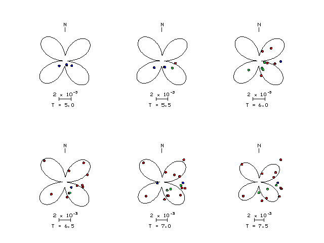
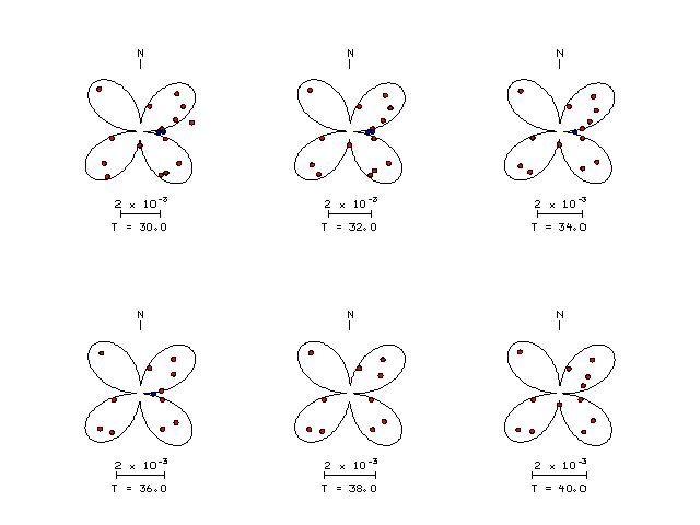
| Pressure-tension axis trends. Since the surface-wave spectra search does not distinguish between P and T axes and since there is a 180 ambiguity in strike, all possible P and T axes are plotted. First motion data and waveforms will be used to select the preferred mechanism. The purpose of this plot is to provide an idea of the possible range of solutions. The P and T-axes for all mechanisms with goodness of fit greater than 0.9 FITMAX (above) are plotted here. |

|
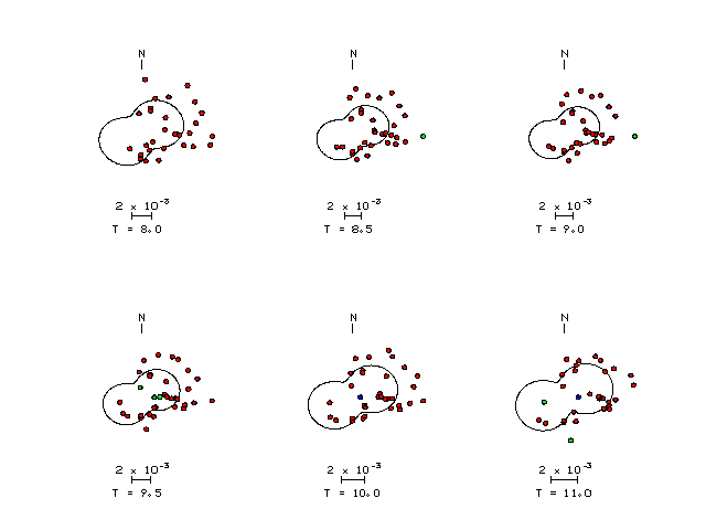
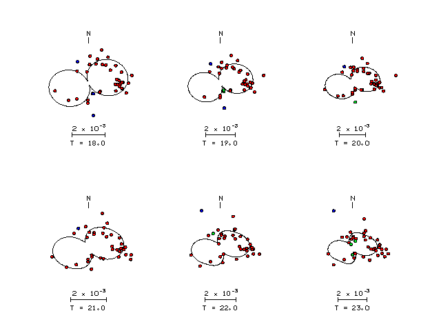
| Focal mechanism sensitivity at the preferred depth. The red color indicates a very good fit to the Love and Rayleigh wave radiation patterns. Each solution is plotted as a vector at a given value of strike and dip with the angle of the vector representing the rake angle, measured, with respect to the upward vertical (N) in the figure. A nearly vertical strike-slip fault striking at 75 or 165 degrees is preferred. Because of the symmetry of the spectral amplitude rediation patterns, only strikes from 0-180 degrees are sampled. |
The P-wave first motion data for focal mechanism studies are as follow:
Sta Az(deg)    Dist(km)   First motion
WVOR	   80	  138	e+
YBH	  256	  209	i+
BEKR	  182	  261	e+
BMN	  127	  324	X
WCN	  172	  326	X
COR	  318	  359	e+
HOPS	  214	  429	X
MNV	  156	  458	X
CMB	  181	  465	X
HLID	   71	  502	X
The P-wave first motion data for focal mechanism studies are as follow:
Sta Az(deg)    Dist(km)
WVOR	   80	  138
YBH	  256	  209
BEKR	  182	  261
WDC	  227	  263
BMN	  127	  324
WCN	  172	  326
COR	  318	  359
HOPS	  214	  429
MNV	  156	  458
CMB	  181	  465
HLID	   71	  502
TPH	  150	  529
HVU	   92	  624
DUG	  107	  665
DAC	  160	  699
NEW	   19	  716
MSO	   42	  718
HWUT	   92	  726
JLU	  101	  759
MPU	  106	  766
PNT	    4	  790
BOZ	   58	  791
BW06	   82	  883
LLLB	  353	  941
WUAZ	  131	 1072
BBB	  335	 1255
EDM	   20	 1328
MOBC	  329	 1496
FNBB	  355	 1864
ULM	   56	 2071
WHY	  339	 2277
UALR	  100	 2560
SLM	   89	 2567
FVM	   90	 2575
FCC	   36	 2584
PVMO	   94	 2699
MPH	   97	 2740
UTMT	   93	 2771
USIN	   89	 2804
BLO	   85	 2854
Since the analysis of the surface-wave radiation patterns uses only spectral amplitudes and because the surfave-wave radiation patterns have a 180 degree symmetry, each surface-wave solution consists of four possible focal mechanisms corresponding to the interchange of the P- and T-axes and a roation of the mechanism by 180 degrees. To select one mechanism, P-wave first motion can be used. This was not possible in this case because all the P-wave first motions were emergent ( a feature of the P-wave wave takeoff angle, the station location and the mechanism). The other way to select among the mechanisms is to compute forward synthetics and compare the observed and predicted waveforms.
The fits to the waveforms with the given mechanism are show below:

|
This figure shows the fit to the three components of motion (Z - vertical, R-radial and T - transverse). For each station and component, the observed traces is shown in red and the model predicted trace in blue. The traces represent filtered ground velocity in units of meters/sec (the peak value is printed adjacent to each trace; each pair of traces to plotted to the same scale to emphasize the difference in levels). Both synthetic and observed traces have been filtered using the SAC commands:
hp c 0.02 3
lp c 0.05 3

|

|
Should the national backbone of the USGS Advanced National Seismic System (ANSS) be implemented with an interstation separation of 300 km, it is very likely that an earthquake such as this would have been recorded at distances on the order of 100-200 km. This means that the closest station would have information on source depth and mechanism that was lacking here.
Dr. Harley Benz, USGS, provided the USGS USNSN digital data.
The figures below show the observed spectral amplitudes (units of cm-sec) at each station and the
theoretical predictions as a function of period for the mechanism given above. The modified Utah model earth model
was used to define the Green's functions. For each station, the Love and Rayleigh wave spectrail amplitudes are plotted with the same scaling so that one can get a sense fo the effects of the effects of the focal mechanism and depth on the excitation of each.
 |
 |
 |
 |
 |
 |
 |
 |
 |
 |
 |
 |
 |
 |
 |
 |
 |
 |
 |
 |
 |
 |
 |
 |
 |
 |
 |
 |
 |
 |
 |
 |
 |
 |
 |
 |
 |
 |
 |
 |
Here we tabulate the reasons for not using certain digital data sets
The following stations did not have a valid response files: