
USGS Felt map for this earthquake
 SLU Moment Tensor Solution


 Best Fitting Double Couple
    Mo = 5.62e+23 dyne-cm
    Mw = 5.10
    Z  = 10 km
     Plane   Strike  Dip  Rake
      NP1      349    47   -105
      NP2      190    45   -75
 Principal Axes:
   Axis    Value   Plunge  Azimuth
     T   5.62e+23      1      89
     N   0.00e+00     11     359
     P  -5.62e+23     79     185


 Moment Tensor: (dyne-cm)
    Component  Value
       Mxx    -1.88e+22
       Mxy     3.82e+21
       Mxz     1.01e+23
       Myy     5.62e+23
       Myz     1.79e+22
       Mzz    -5.43e+23


                     ######--######
                 #########----#########
              ##########--------##########
             #########-----------##########
           ##########--------------##########
          ##########----------------##########
         ##########------------------##########
        ##########-------------------###########
        ##########--------------------##########
       ##########---------------------#########
       ##########----------------------######## T
       ##########---------   ----------########
       ##########--------- P ----------##########
        #########---------   ----------#########
        #########----------------------#########
         ########----------------------########
          ########--------------------########
           #######--------------------#######
             ######------------------######
              ######----------------######
                 ####--------------####
                     ##----------##


 Harvard Convention
 Moment Tensor:
      R          T          F
 -5.43e+23   1.01e+23  -1.79e+22
  1.01e+23  -1.88e+22  -3.82e+21
 -1.79e+22  -3.82e+21   5.62e+23


Details of the solution is found at

http://www.eas.slu.edu/eqc/eqc_mt/MECH.NA//index.html
|
Normal fault CMT 042101E EASTERN IDAHO Date: 2001/ 4/21 Centroid Time: 17:19: 2.4 GMT Lat= 43.02 Lon=-111.29 Depth= 15.0 Half duration= 1.1 Centroid time minus hypocenter time: 5.4 Moment Tensor: Expo=24 -1.050 0.030 1.020 -0.170 0.110 0.040 Mw = 5.3 mb = 5.4 Ms = 4.9 Scalar Moment = 1.05e+24 Fault plane: strike=11 dip=43 slip=-77 Fault plane: strike=173 dip=48 slip=-102 |
      STK = 190
      DIP = 45
     RAKE = -75
       MW = 5.10
       HS = 10
The waveform inversion is preferred. The surface-eave solution is equivalent.
The following compares this source inversion to others
The focal mechanism was determined using broadband seismic waveforms. The location of the event and the and stations used for the waveform inversion are shown in the next figure.
|
|
|
|
The program wvfgrd96 was used with good traces observed at short distance to determine the focal mechanism, depth and seismic moment. This technique requires a high quality signal and well determined velocity model for the Green functions. To the extent that these are the quality data, this type of mechanism should be preferred over the radiation pattern technique which requires the separate step of defining the pressure and tension quadrants and the correct strike.
The observed and predicted traces are filtered using the following gsac commands:
hp c 0.01 n 3
lp c 0.05 n 3
The results of this grid search from 0.5 to 19 km depth are as follow:
           DEPTH  STK   DIP  RAKE   MW    FIT
WVFGRD96    0.5   220    90   -15   4.59 0.1806
WVFGRD96    1.0   220    90   -10   4.62 0.1929
WVFGRD96    2.0   220    90   -10   4.70 0.2182
WVFGRD96    3.0   220    75   -25   4.79 0.2330
WVFGRD96    4.0   220    80   -50   4.89 0.2619
WVFGRD96    5.0   215    70   -50   4.92 0.3107
WVFGRD96    6.0   205    55   -55   4.96 0.3766
WVFGRD96    7.0   200    50   -65   5.01 0.4382
WVFGRD96    8.0   200    50   -65   5.08 0.4935
WVFGRD96    9.0   200    50   -65   5.10 0.5410
WVFGRD96   10.0   190    45   -75   5.10 0.5578
WVFGRD96   11.0   200    50   -65   5.09 0.5493
WVFGRD96   12.0   200    50   -65   5.08 0.5291
WVFGRD96   13.0   200    50   -60   5.06 0.5032
WVFGRD96   14.0    35    55   -35   5.05 0.4806
WVFGRD96   15.0    45    70   -15   5.08 0.4642
WVFGRD96   16.0    45    70   -15   5.08 0.4499
WVFGRD96   17.0    45    75   -10   5.09 0.4354
WVFGRD96   18.0    45    75   -10   5.08 0.4200
WVFGRD96   19.0    45    80    -5   5.09 0.4023
WVFGRD96   20.0    45    80    -5   5.09 0.3861
WVFGRD96   21.0    45    80    -5   5.09 0.3702
WVFGRD96   22.0   225    90     5   5.10 0.3580
WVFGRD96   23.0   225    90    10   5.10 0.3510
WVFGRD96   24.0   225    90    10   5.10 0.3437
WVFGRD96   25.0   225    90    10   5.10 0.3366
WVFGRD96   26.0   225    90    10   5.10 0.3269
WVFGRD96   27.0   225    90    10   5.10 0.3192
WVFGRD96   28.0   225    85    10   5.10 0.3094
WVFGRD96   29.0   225    85    10   5.11 0.3014
The best solution is
WVFGRD96 10.0 190 45 -75 5.10 0.5578
The mechanism correspond to the best fit is

|
|
|
The best fit as a function of depth is given in the following figure:

|
|
|
The comparison of the observed and predicted waveforms is given in the next figure. The red traces are the observed and the blue are the predicted. Each observed-predicted componnet is plotted to the same scale and peak amplitudes are indicated by the numbers to the left of each trace. The number in black at the rightr of each predicted traces it the time shift required for maximum correlation between the observed and predicted traces. This time shift is required because the synthetics are not computed at exactly the same distance as the observed and because the velocity model used in the predictions may not be perfect. A positive time shift indicates that the prediction is too fast and should be delayed to match the observed trace (shift to the right in this figure). A negative value indicates that the prediction is too slow. The bandpass filter used in the processing and for the display was
hp c 0.01 n 3
lp c 0.05 n 3

|
|
|

|
| Focal mechanism sensitivity at the preferred depth. The red color indicates a very good fit to thewavefroms. Each solution is plotted as a vector at a given value of strike and dip with the angle of the vector representing the rake angle, measured, with respect to the upward vertical (N) in the figure. |
The following figure shows the stations used in the grid search for the best focal mechanism to fit the surface-wave spectral amplitudes of the Love and Rayleigh waves.

|
|
|
The surface-wave determined focal mechanism is shown here.
  NODAL PLANES


  STK=     194.25
  DIP=      51.62
 RAKE=     -77.75

             OR

  STK=     354.97
  DIP=      40.00
 RAKE=    -105.00


DEPTH = 10.0 km

Mw = 5.22
Best Fit 0.9010 - P-T axis plot gives solutions with FIT greater than FIT90
 |
The P-wave first motion data for focal mechanism studies are as follow:
Sta Az(deg)    Dist(km)   First motion
HWUT      186  147 iP_D
BW06       95  151 eP_C
HLID      287  256 iP_C
BOZ       356  304 iP_D
DUG       202  325 iP_D
ELK       234  401 iP_D
MVU       188  495 iP_D
Surface wave analysis was performed using codes from Computer Programs in Seismology, specifically the multiple filter analysis program do_mft and the surface-wave radiation pattern search program srfgrd96.
Digital data were collected, instrument response removed and traces converted
to Z, R an T components. Multiple filter analysis was applied to the Z and T traces to obtain the Rayleigh- and Love-wave spectral amplitudes, respectively.
These were input to the search program which examined all depths between 1 and 25 km
and all possible mechanisms.

|
|
|

|
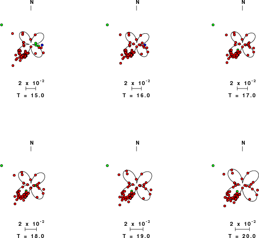
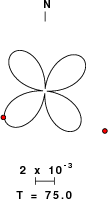
| Pressure-tension axis trends. Since the surface-wave spectra search does not distinguish between P and T axes and since there is a 180 ambiguity in strike, all possible P and T axes are plotted. First motion data and waveforms will be used to select the preferred mechanism. The purpose of this plot is to provide an idea of the possible range of solutions. The P and T-axes for all mechanisms with goodness of fit greater than 0.9 FITMAX (above) are plotted here. |

|
| Focal mechanism sensitivity at the preferred depth. The red color indicates a very good fit to the Love and Rayleigh wave radiation patterns. Each solution is plotted as a vector at a given value of strike and dip with the angle of the vector representing the rake angle, measured, with respect to the upward vertical (N) in the figure. Because of the symmetry of the spectral amplitude rediation patterns, only strikes from 0-180 degrees are sampled. |
The distribution of broadband stations with azimuth and distance is
Sta Az(deg)    Dist(km)
HWUT	  186	  147
BW06	   95	  151
HLID	  287	  256
BOZ	  356	  304
DUG	  202	  325
ELK	  234	  401
MVU	  188	  495
BMN	  242	  559
ISCO	  124	  595
WVOR	  267	  596
RSSD	   75	  609
TPH	  224	  730
NEW	  325	  743
PAHR	  245	  758
PIN	  281	  774
WCN	  243	  808
MLAC	  230	  863
TIN	  224	  874
DAC	  218	  909
CWC	  221	  920
MPM	  216	  924
LON	  301	  926
CMB	  238	  935
WDC	  258	  962
DBO	  275	  966
GSC	  211	  966
COR	  285	  976
ANMO	  153	  982
DAN	  202	  982
ISA	  220	 1010
GNW	  304	 1034
SQM	  306	 1075
CBKS	  111	 1082
SVD	  209	 1097
SAO	  235	 1098
OSI	  217	 1120
KNW	  206	 1122
PFO	  205	 1124
MWC	  213	 1126
SND	  205	 1135
WMC	  206	 1135
GLA	  196	 1136
RDM	  207	 1136
CRY	  206	 1138
PAS	  213	 1138
DGR	  207	 1140
FRD	  205	 1141
BZN	  206	 1143
PHL	  226	 1148
LVA2	  205	 1154
DJJ	  214	 1155
USC	  214	 1156
PLM	  206	 1164
TOV	  216	 1168
LLLB	  321	 1169
TUC	  177	 1179
JCS	  204	 1183
SBC	  220	 1186
RPV	  213	 1188
MONP	  203	 1197
CIA	  212	 1222
BAR	  204	 1227
SOL	  207	 1231
SNCC	  216	 1288
FFC	   24	 1481
CCM	  101	 1786
SLM	   98	 1842
UALR	  112	 1878
SIUC	  100	 1965
MPH	  108	 2042
BLO	   93	 2124
YKW3	  356	 2196
SSPA	   84	 2778
Since the analysis of the surface-wave radiation patterns uses only spectral amplitudes and because the surfave-wave radiation patterns have a 180 degree symmetry, each surface-wave solution consists of four possible focal mechanisms corresponding to the interchange of the P- and T-axes and a roation of the mechanism by 180 degrees. To select one mechanism, P-wave first motion can be used. This was not possible in this case because all the P-wave first motions were emergent ( a feature of the P-wave wave takeoff angle, the station location and the mechanism). The other way to select among the mechanisms is to compute forward synthetics and compare the observed and predicted waveforms.
The fits to the waveforms with the given mechanism are show below:

|
This figure shows the fit to the three components of motion (Z - vertical, R-radial and T - transverse). For each station and component, the observed traces is shown in red and the model predicted trace in blue. The traces represent filtered ground velocity in units of meters/sec (the peak value is printed adjacent to each trace; each pair of traces to plotted to the same scale to emphasize the difference in levels). Both synthetic and observed traces have been filtered using the SAC commands:
hp c 0.01 n 3
lp c 0.05 n 3

|

|
Should the national backbone of the USGS Advanced National Seismic System (ANSS) be implemented with an interstation separation of 300 km, it is very likely that an earthquake such as this would have been recorded at distances on the order of 100-200 km. This means that the closest station would have information on source depth and mechanism that was lacking here.
Dr. Harley Benz, USGS, provided the USGS USNSN digital data. The digital data used in this study were provided by Natural Resources Canada through their AUTODRM site http://www.seismo.nrcan.gc.ca/nwfa/autodrm/autodrm_req_e.php, and IRIS using their BUD interface.
Thanks also to the many seismic network operators whose dedication make this effort possible: University of Alaska, University of Washington, Oregon State University, University of Utah, Montana Bureas of Mines, UC Berkely, Caltech, UC San Diego, Saint L ouis University, Universityof Memphis, Lamont Doehrty Earth Observatory, Boston College, the Iris stations and the Transportable Array of EarthScope.
The WUS used for the waveform synthetic seismograms and for the surface wave eigenfunctions and dispersion is as follows:
MODEL.01
Model after     8 iterations
ISOTROPIC
KGS
FLAT EARTH
1-D
CONSTANT VELOCITY
LINE08
LINE09
LINE10
LINE11
      H(KM)   VP(KM/S)   VS(KM/S) RHO(GM/CC)         QP         QS       ETAP       ETAS      FREFP      FREFS
     1.9000     3.4065     2.0089     2.2150  0.302E-02  0.679E-02   0.00       0.00       1.00       1.00
     6.1000     5.5445     3.2953     2.6089  0.349E-02  0.784E-02   0.00       0.00       1.00       1.00
    13.0000     6.2708     3.7396     2.7812  0.212E-02  0.476E-02   0.00       0.00       1.00       1.00
    19.0000     6.4075     3.7680     2.8223  0.111E-02  0.249E-02   0.00       0.00       1.00       1.00
     0.0000     7.9000     4.6200     3.2760  0.164E-10  0.370E-10   0.00       0.00       1.00       1.00
Here we tabulate the reasons for not using certain digital data sets
The following stations did not have a valid response files:
DATE=Tue Nov 13 14:15:13 CST 2007