2014/03/31 19:48:35 36.95 124.50 10.0 5.1 Korea
USGS Felt map for this earthquake
 USGS/SLU Moment Tensor Solution
 ENS  2014/03/31 19:48:35:0  36.95  124.50  10.0 5.1 Korea

 Stations used:
   KS.BAR KS.BUS KS.BUS2 KS.CHJ KS.DACB KS.DAG2 KS.DGY2
   KS.GAHB KS.HWCB KS.JJU KS.KOHB KS.KWJ KS.SEHB KS.SEO
   KS.SEO2

 Filtering commands used:
   hp c 0.02 n 3
   lp c 0.10 n 3

 Best Fitting Double Couple
  Mo = 1.62e+23 dyne-cm
  Mw = 4.74
  Z  = 12 km
  Plane   Strike  Dip  Rake
   NP1      115    60   -45
   NP2      232    52   -141
  Principal Axes:
   Axis    Value   Plunge  Azimuth
    T   1.62e+23      5     175
    N   0.00e+00     38     268
    P  -1.62e+23     52      79

 Moment Tensor: (dyne-cm)
    Component   Value
       Mxx     1.58e+23
       Mxy    -2.58e+22
       Mxz    -2.77e+22
       Myy    -5.83e+22
       Myz    -7.62e+22
       Mzz    -9.93e+22


                     ##############
                 ######################
              ############################
             ##############################
           ###################---------------
          ################--------------------
         ##############------------------------
        --###########---------------------------
        ---########-----------------------------
       -----#####-------------------   ----------
       -------##-------------------- P ----------
       --------#--------------------   ----------
       -------####-------------------------------
        -----########---------------------------
        ----############------------------------
         ---################-------------------
          --#########################----#####
           -#################################
             ##############################
              ############################
                 ###########   ########
                     ####### T ####


 Global CMT Convention Moment Tensor:
      R          T          P
 -9.93e+22  -2.77e+22   7.62e+22
 -2.77e+22   1.58e+23   2.58e+22
  7.62e+22   2.58e+22  -5.83e+22


Details of the solution is found at

http://www.eas.slu.edu/eqc/eqc_mt/MECH.NA/20140331194835/index.html
|
      STK = 115
      DIP = 60
     RAKE = -45
       MW = 4.74
       HS = 12.0
The waveform inversion is preferred.
The following compares this source inversion to others
 USGS/SLU Moment Tensor Solution
 ENS  2014/03/31 19:48:35:0  36.95  124.50  10.0 5.1 Korea

 Stations used:
   KS.BAR KS.BUS KS.BUS2 KS.CHJ KS.DACB KS.DAG2 KS.DGY2
   KS.GAHB KS.HWCB KS.JJU KS.KOHB KS.KWJ KS.SEHB KS.SEO
   KS.SEO2

 Filtering commands used:
   hp c 0.02 n 3
   lp c 0.10 n 3

 Best Fitting Double Couple
  Mo = 1.62e+23 dyne-cm
  Mw = 4.74
  Z  = 12 km
  Plane   Strike  Dip  Rake
   NP1      115    60   -45
   NP2      232    52   -141
  Principal Axes:
   Axis    Value   Plunge  Azimuth
    T   1.62e+23      5     175
    N   0.00e+00     38     268
    P  -1.62e+23     52      79

 Moment Tensor: (dyne-cm)
    Component   Value
       Mxx     1.58e+23
       Mxy    -2.58e+22
       Mxz    -2.77e+22
       Myy    -5.83e+22
       Myz    -7.62e+22
       Mzz    -9.93e+22


                     ##############
                 ######################
              ############################
             ##############################
           ###################---------------
          ################--------------------
         ##############------------------------
        --###########---------------------------
        ---########-----------------------------
       -----#####-------------------   ----------
       -------##-------------------- P ----------
       --------#--------------------   ----------
       -------####-------------------------------
        -----########---------------------------
        ----############------------------------
         ---################-------------------
          --#########################----#####
           -#################################
             ##############################
              ############################
                 ###########   ########
                     ####### T ####


 Global CMT Convention Moment Tensor:
      R          T          P
 -9.93e+22  -2.77e+22   7.62e+22
 -2.77e+22   1.58e+23   2.58e+22
  7.62e+22   2.58e+22  -5.83e+22


Details of the solution is found at

http://www.eas.slu.edu/eqc/eqc_mt/MECH.NA/20140331194835/index.html
|
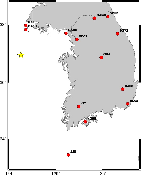
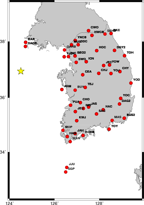
The focal mechanism was determined using broadband seismic waveforms. The location of the event and the and stations used for the waveform inversion are shown in the next figure.
|
|
|
|
The program wvfgrd96 was used with good traces observed at short distance to determine the focal mechanism, depth and seismic moment. This technique requires a high quality signal and well determined velocity model for the Green functions. To the extent that these are the quality data, this type of mechanism should be preferred over the radiation pattern technique which requires the separate step of defining the pressure and tension quadrants and the correct strike.
The observed and predicted traces are filtered using the following gsac commands:
hp c 0.02 n 3
lp c 0.10 n 3
The results of this grid search from 0.5 to 19 km depth are as follow:
           DEPTH  STK   DIP  RAKE   MW    FIT
WVFGRD96    0.5   300    50    80   4.51 0.5801
WVFGRD96    1.0   310    45    80   4.57 0.5731
WVFGRD96    2.0   120    70    65   4.64 0.5450
WVFGRD96    3.0   135    65    60   4.67 0.5606
WVFGRD96    4.0   120    70    60   4.64 0.5631
WVFGRD96    5.0   120    85   -50   4.62 0.5872
WVFGRD96    6.0   110    65   -55   4.67 0.6554
WVFGRD96    7.0   100    55   -65   4.72 0.7232
WVFGRD96    8.0   105    55   -60   4.72 0.7733
WVFGRD96    9.0   105    55   -55   4.72 0.8038
WVFGRD96   10.0   110    55   -50   4.73 0.8220
WVFGRD96   11.0   110    55   -50   4.74 0.8308
WVFGRD96   12.0   115    60   -45   4.74 0.8333
WVFGRD96   13.0   115    60   -45   4.75 0.8293
WVFGRD96   14.0   115    60   -45   4.75 0.8196
WVFGRD96   15.0   115    60   -45   4.76 0.8065
WVFGRD96   16.0   115    60   -45   4.77 0.7902
WVFGRD96   17.0   115    55   -40   4.79 0.7740
WVFGRD96   18.0   120    60   -35   4.81 0.7568
WVFGRD96   19.0   120    55   -35   4.82 0.7388
WVFGRD96   20.0   120    55   -35   4.83 0.7196
WVFGRD96   21.0   120    55   -35   4.84 0.7010
WVFGRD96   22.0   120    55   -35   4.85 0.6819
WVFGRD96   23.0   120    55   -30   4.86 0.6613
WVFGRD96   24.0   120    55   -30   4.87 0.6402
WVFGRD96   25.0   120    55   -30   4.88 0.6188
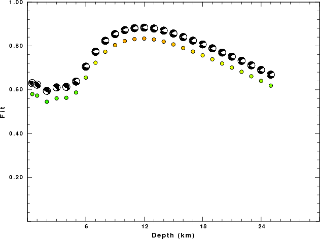
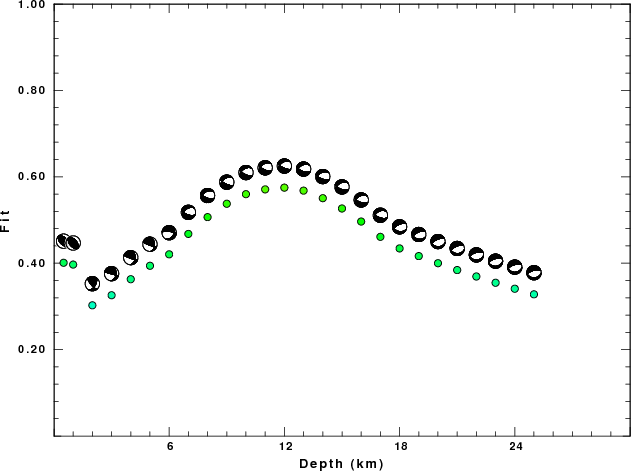
The best solution is
WVFGRD96 12.0 115 60 -45 4.74 0.8333
The mechanism correspond to the best fit is
|
|
|
The best fit as a function of depth is given in the following figure:
|
|
|
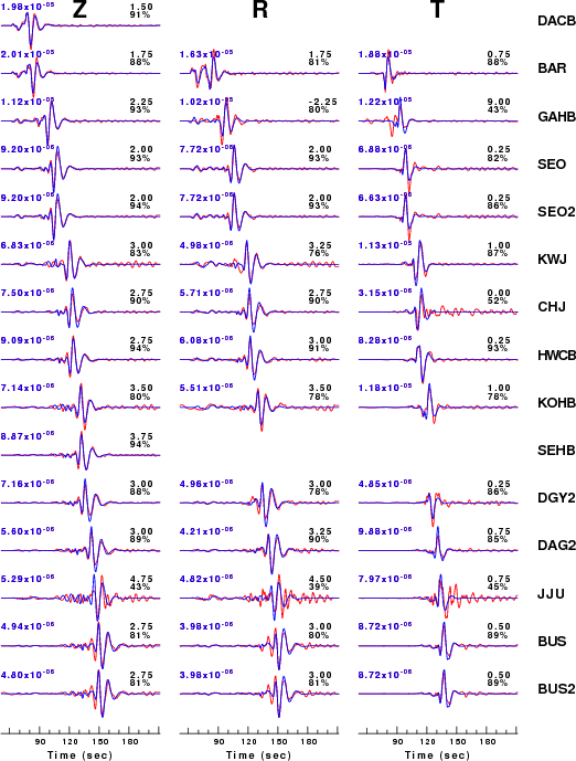
The comparison of the observed and predicted waveforms is given in the next figure. The red traces are the observed and the blue are the predicted. Each observed-predicted component is plotted to the same scale and peak amplitudes are indicated by the numbers to the left of each trace. A pair of numbers is given in black at the right of each predicted traces. The upper number it the time shift required for maximum correlation between the observed and predicted traces. This time shift is required because the synthetics are not computed at exactly the same distance as the observed and because the velocity model used in the predictions may not be perfect. A positive time shift indicates that the prediction is too fast and should be delayed to match the observed trace (shift to the right in this figure). A negative value indicates that the prediction is too slow. The lower number gives the percentage of variance reduction to characterize the individual goodness of fit (100% indicates a perfect fit).
The bandpass filter used in the processing and for the display was
hp c 0.02 n 3
lp c 0.10 n 3
|
|
|
|
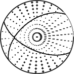
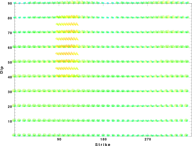
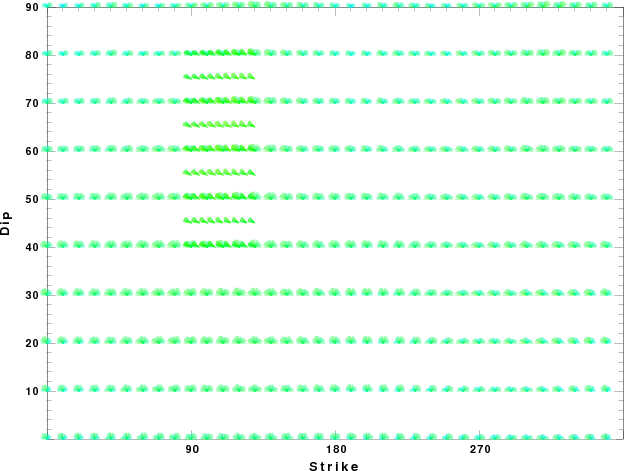
| Focal mechanism sensitivity at the preferred depth. The red color indicates a very good fit to thewavefroms. Each solution is plotted as a vector at a given value of strike and dip with the angle of the vector representing the rake angle, measured, with respect to the upward vertical (N) in the figure. |
A check on the assumed source location is possible by looking at the time shifts between the observed and predicted traces. The time shifts for waveform matching arise for several reasons:
Time_shift = A + B cos Azimuth + C Sin Azimuth
The time shifts for this inversion lead to the next figure:
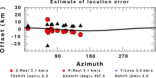
The derived shift in origin time and epicentral coordinates are given at the bottom of the figure.
The focal mechanism was determined using broadband seismic waveforms. The location of the event and the and stations used for the waveform inversion are shown in the next figure.
|
|
|
The program wvfgrd96 was used with good traces observed at short distance to determine the focal mechanism, depth and seismic moment. This technique requires a high quality signal and well determined velocity model for the Green functions. To the extent that these are the quality data, this type of mechanism should be preferred over the radiation pattern technique which requires the separate step of defining the pressure and tension quadrants and the correct strike.
The observed and predicted traces are filtered using the following gsac commands:
hp c 0.04 n 3
lp c 0.20 n 3
The results of this grid search from 0.5 to 19 km depth are as follow:
           DEPTH  STK   DIP  RAKE   MW    FIT
WVFGRD96    0.5   135    45    90   4.43 0.4011
WVFGRD96    1.0   140    45    90   4.51 0.3969
WVFGRD96    2.0   140    70    45   4.46 0.3026
WVFGRD96    3.0   105    85    55   4.45 0.3259
WVFGRD96    4.0   110    80    55   4.48 0.3630
WVFGRD96    5.0   110    75    60   4.50 0.3941
WVFGRD96    6.0   275    75   -60   4.53 0.4206
WVFGRD96    7.0   110    60   -55   4.59 0.4679
WVFGRD96    8.0   110    60   -60   4.63 0.5067
WVFGRD96    9.0   115    65   -55   4.65 0.5377
WVFGRD96   10.0   115    65   -55   4.67 0.5599
WVFGRD96   11.0   115    65   -55   4.69 0.5709
WVFGRD96   12.0   115    65   -55   4.72 0.5750
WVFGRD96   13.0   110    60   -60   4.74 0.5680
WVFGRD96   14.0   110    60   -60   4.76 0.5506
WVFGRD96   15.0   110    60   -60   4.77 0.5267
WVFGRD96   16.0   110    60   -60   4.77 0.4965
WVFGRD96   17.0   110    60   -60   4.79 0.4611
WVFGRD96   18.0   105    35   -55   4.80 0.4343
WVFGRD96   19.0   105    35   -55   4.81 0.4165
WVFGRD96   20.0    95    30   -65   4.82 0.4001
WVFGRD96   21.0    95    30   -65   4.83 0.3842
WVFGRD96   22.0    90    30   -75   4.85 0.3693
WVFGRD96   23.0    85    30   -80   4.86 0.3548
WVFGRD96   24.0    90    30   -75   4.87 0.3410
WVFGRD96   25.0    90    30   -75   4.87 0.3280
The best solution is
WVFGRD96 12.0 115 65 -55 4.72 0.5750
The mechanism correspond to the best fit is

|
|
|
The best fit as a function of depth is given in the following figure:
|
|
|
The comparison of the observed and predicted waveforms is given in the next figure. The red traces are the observed and the blue are the predicted. Each observed-predicted component is plotted to the same scale and peak amplitudes are indicated by the numbers to the left of each trace. A pair of numbers is given in black at the right of each predicted traces. The upper number it the time shift required for maximum correlation between the observed and predicted traces. This time shift is required because the synthetics are not computed at exactly the same distance as the observed and because the velocity model used in the predictions may not be perfect. A positive time shift indicates that the prediction is too fast and should be delayed to match the observed trace (shift to the right in this figure). A negative value indicates that the prediction is too slow. The lower number gives the percentage of variance reduction to characterize the individual goodness of fit (100% indicates a perfect fit).
The bandpass filter used in the processing and for the display was
hp c 0.04 n 3
lp c 0.20 n 3

|
|
|
|
| Focal mechanism sensitivity at the preferred depth. The red color indicates a very good fit to thewavefroms. Each solution is plotted as a vector at a given value of strike and dip with the angle of the vector representing the rake angle, measured, with respect to the upward vertical (N) in the figure. |
Thanks also to the many seismic network operators whose dedication make this effort possible: University of Nevada Reno, University of Alaska, University of Washington, Oregon State University, University of Utah, Montana Bureas of Mines, UC Berkely, Caltech, UC San Diego, Saint Louis University, University of Memphis, Lamont Doherty Earth Observatory, the Iris stations and the Transportable Array of EarthScope.
The t6.invSNU.CUVEL used for the waveform synthetic seismograms and for the surface wave eigenfunctions and dispersion is as follows:
MODEL.01
Model after    30 iterations
ISOTROPIC
KGS
SPHERICAL EARTH
1-D
CONSTANT VELOCITY
LINE08
LINE09
LINE10
LINE11
      H(KM)   VP(KM/S)   VS(KM/S) RHO(GM/CC)         QP         QS       ETAP       ETAS      FREFP      FREFS
     1.0000     5.3800     3.0009     2.5772  0.118E-02  0.167E-02   0.00       0.00       1.00       1.00
     1.0000     5.8057     3.2383     2.6606  0.118E-02  0.167E-02   0.00       0.00       1.00       1.00
     1.0000     6.1732     3.4433     2.7513  0.118E-02  0.167E-02   0.00       0.00       1.00       1.00
     3.0000     6.2872     3.5067     2.7862  0.118E-02  0.167E-02   0.00       0.00       1.00       1.00
     5.0000     6.3245     3.5281     2.7970  0.118E-02  0.167E-02   0.00       0.00       1.00       1.00
     5.0000     6.4165     3.5788     2.8248  0.118E-02  0.167E-02   0.00       0.00       1.00       1.00
     4.0000     6.5576     3.6576     2.8653  0.118E-02  0.167E-02   0.00       0.00       1.00       1.00
     5.0000     6.6402     3.7038     2.8865  0.118E-02  0.167E-02   0.00       0.00       1.00       1.00
     2.5000     6.6540     3.7115     2.8897  0.118E-02  0.167E-02   0.00       0.00       1.00       1.00
     2.5000     7.0960     3.9579     3.0111  0.118E-02  0.167E-02   0.00       0.00       1.00       1.00
     2.5000     7.9155     4.4148     3.2804  0.118E-02  0.167E-02   0.00       0.00       1.00       1.00
     2.5000     7.8925     4.4019     3.2735  0.118E-02  0.167E-02   0.00       0.00       1.00       1.00
     5.0000     7.8665     4.3876     3.2643  0.118E-02  0.167E-02   0.00       0.00       1.00       1.00
     5.0000     7.5675     4.2211     3.1625  0.118E-02  0.167E-02   0.00       0.00       1.00       1.00
     5.0000     7.7550     4.3252     3.2262  0.118E-02  0.167E-02   0.00       0.00       1.00       1.00
     5.0000     7.7602     4.3280     3.2282  0.118E-02  0.167E-02   0.00       0.00       1.00       1.00
     5.0000     7.7958     4.3487     3.2398  0.118E-02  0.167E-02   0.00       0.00       1.00       1.00
     5.0000     7.7415     4.3195     3.2217  0.118E-02  0.167E-02   0.00       0.00       1.00       1.00
     5.0000     7.6497     4.2688     3.1915  0.118E-02  0.167E-02   0.00       0.00       1.00       1.00
     5.0000     7.6408     4.2653     3.1889  0.118E-02  0.167E-02   0.00       0.00       1.00       1.00
     5.0000     7.6666     4.2716     3.1976  0.118E-02  0.167E-02   0.00       0.00       1.00       1.00
     5.0000     7.6699     4.2830     3.1986  0.118E-02  0.167E-02   0.00       0.00       1.00       1.00
     5.0000     7.6780     4.2885     3.2014  0.118E-02  0.167E-02   0.00       0.00       1.00       1.00
     5.0000     7.6816     4.2896     3.2028  0.118E-02  0.167E-02   0.00       0.00       1.00       1.00
     5.0000     7.6946     4.2996     3.2072  0.118E-02  0.167E-02   0.00       0.00       1.00       1.00
    10.0000     7.7349     4.3197     3.2208  0.118E-02  0.167E-02   0.00       0.00       1.00       1.00
    10.0000     7.7791     4.3484     3.2355  0.118E-02  0.167E-02   0.00       0.00       1.00       1.00
    10.0000     7.8331     4.3722     3.2536  0.862E-02  0.131E-01   0.00       0.00       1.00       1.00
    10.0000     7.8824     4.3863     3.2703  0.862E-02  0.131E-01   0.00       0.00       1.00       1.00
    10.0000     7.9360     4.4024     3.2883  0.855E-02  0.131E-01   0.00       0.00       1.00       1.00
    10.0000     7.9967     4.4237     3.3088  0.847E-02  0.131E-01   0.00       0.00       1.00       1.00
    10.0000     8.0529     4.4423     3.3289  0.847E-02  0.131E-01   0.00       0.00       1.00       1.00
    10.0000     8.1110     4.4603     3.3496  0.833E-02  0.130E-01   0.00       0.00       1.00       1.00
    10.0000     8.1762     4.4832     3.3728  0.826E-02  0.129E-01   0.00       0.00       1.00       1.00
    10.0000     8.2410     4.5054     3.3959  0.813E-02  0.128E-01   0.00       0.00       1.00       1.00
    10.0000     8.3022     4.5257     3.4176  0.806E-02  0.126E-01   0.00       0.00       1.00       1.00
    10.0000     8.3635     4.5514     3.4395  0.474E-02  0.746E-02   0.00       0.00       1.00       1.00
    10.0000     8.4257     4.5839     3.4617  0.472E-02  0.741E-02   0.00       0.00       1.00       1.00
    10.0000     8.4845     4.6145     3.4827  0.469E-02  0.741E-02   0.00       0.00       1.00       1.00
    10.0000     8.5403     4.6434     3.5020  0.467E-02  0.735E-02   0.00       0.00       1.00       1.00
    10.0000     8.5934     4.6708     3.5199  0.465E-02  0.735E-02   0.00       0.00       1.00       1.00
    10.0000     8.6436     4.6959     3.5369  0.463E-02  0.730E-02   0.00       0.00       1.00       1.00
    10.0000     8.6912     4.7194     3.5530  0.461E-02  0.730E-02   0.00       0.00       1.00       1.00
    10.0000     8.7365     4.7413     3.5684  0.459E-02  0.725E-02   0.00       0.00       1.00       1.00
    10.0000     8.7797     4.7622     3.5831  0.455E-02  0.725E-02   0.00       0.00       1.00       1.00
    10.0000     8.8199     4.7819     3.5967  0.452E-02  0.719E-02   0.00       0.00       1.00       1.00
    10.0000     8.8587     4.8001     3.6099  0.450E-02  0.714E-02   0.00       0.00       1.00       1.00
    10.0000     8.8958     4.8177     3.6226  0.448E-02  0.714E-02   0.00       0.00       1.00       1.00
    10.0000     8.9314     4.8346     3.6347  0.446E-02  0.709E-02   0.00       0.00       1.00       1.00
    10.0000     8.9647     4.8500     3.6461  0.442E-02  0.704E-02   0.00       0.00       1.00       1.00
    10.0000     8.9962     4.8651     3.6569  0.441E-02  0.704E-02   0.00       0.00       1.00       1.00
    10.0000     9.0263     4.8783     3.6685  0.439E-02  0.699E-02   0.00       0.00       1.00       1.00
    10.0000     9.0547     4.8915     3.6800  0.435E-02  0.694E-02   0.00       0.00       1.00       1.00
    10.0000     9.0822     4.9041     3.6911  0.433E-02  0.690E-02   0.00       0.00       1.00       1.00
    10.0000     9.1091     4.9164     3.7020  0.431E-02  0.690E-02   0.00       0.00       1.00       1.00
    10.0000     9.1346     4.9280     3.7123  0.427E-02  0.685E-02   0.00       0.00       1.00       1.00
    10.0000     9.4876     5.1513     3.8537  0.388E-02  0.613E-02   0.00       0.00       1.00       1.00
    10.0000     9.5095     5.1663     3.8624  0.388E-02  0.613E-02   0.00       0.00       1.00       1.00
    10.0000     9.5299     5.1806     3.8703  0.386E-02  0.610E-02   0.00       0.00       1.00       1.00
    10.0000     9.5507     5.1944     3.8784  0.386E-02  0.610E-02   0.00       0.00       1.00       1.00
    10.0000     9.5706     5.2080     3.8861  0.385E-02  0.606E-02   0.00       0.00       1.00       1.00
    10.0000     9.5900     5.2214     3.8937  0.385E-02  0.606E-02   0.00       0.00       1.00       1.00
    10.0000     9.6090     5.2347     3.9011  0.383E-02  0.606E-02   0.00       0.00       1.00       1.00
    10.0000     9.6272     5.2480     3.9081  0.383E-02  0.602E-02   0.00       0.00       1.00       1.00
    10.0000     9.6458     5.2604     3.9154  0.383E-02  0.602E-02   0.00       0.00       1.00       1.00
    10.0000     9.6794     5.2816     3.9282  0.382E-02  0.599E-02   0.00       0.00       1.00       1.00
    10.0000     9.7130     5.3029     3.9409  0.382E-02  0.599E-02   0.00       0.00       1.00       1.00
    10.0000     9.7466     5.3242     3.9537  0.380E-02  0.599E-02   0.00       0.00       1.00       1.00
    10.0000     9.7799     5.3454     3.9664  0.380E-02  0.595E-02   0.00       0.00       1.00       1.00
    10.0000     9.8137     5.3669     3.9792  0.380E-02  0.595E-02   0.00       0.00       1.00       1.00
    10.0000     9.8473     5.3883     3.9920  0.379E-02  0.592E-02   0.00       0.00       1.00       1.00
    10.0000     9.8808     5.4094     4.0047  0.379E-02  0.592E-02   0.00       0.00       1.00       1.00
     0.0000     9.9144     5.4306     4.0175  0.377E-02  0.592E-02   0.00       0.00       1.00       1.00
Here we tabulate the reasons for not using certain digital data sets
The following stations did not have a valid response files: