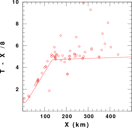
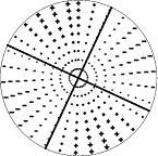
Reduced travel time plot of first arrivals
2007/01/20 11:56:53 37.68N 128.59E 8 4.55 Korea - SLU (below)
2007 01 20 11 56 54 330 37.643 128.472 10.0 4.4 USGS
2007 01 20 11 56 51 000 37.75  128.69  10.0 4.8 KNEIC

SLU Elocate solution using P and S at distances less than 100 km
2007 01 20 11 56 53 874  37.687 128.584 7.37 4.4 KOREA RBH - acc stations
 Error Ellipse  X=   0.3419 km  Y= 0.4248 km  Theta =  99.7164 deg

 RMS Error        :               0.150              sec
 Travel_Time_Table:          KOREA
 Latitude         :             37.6869 +-    0.0038 N         0.4227 km
 Longitude        :            128.5841 +-    0.0039 E         0.3446 km
 Depth            :                7.37 +-      0.71 km
 Epoch Time       :      1169294213.874 +-      0.05 sec
 Event Time       :  20070120115653.874 +-      0.05 sec
 HYPO71 Quality   :                  CB
 Gap              :                  81              deg

 81 phases used

 STA  COMP DIS(K) AZM  AIN    ARR TIME             RES(SEC) WT QFM PHASE    WGT
 DGY    Z    7.95  87. 131. 20070120115655.734         0.08  0 iD P        0.86
 DGY    Z    7.95  87. 131. 20070120115657.274         0.21  0 iX S        0.69
 KAN    Z   27.57  77. 102. 20070120115658.444        -0.08  0 iD P        0.86
 KAN    Z   27.57  77. 101. 20070120115701.932        -0.27  2 eX S        0.31
 JES    Z   29.42 166. 101. 20070120115658.715        -0.09  0 iC P        0.84
 JES    Z   29.42 166. 100. 20070120115703.003         0.29  2 eX S        0.30
 TOH    Z   51.72 113.  95. 20070120115702.306        -0.01  0 iD P        0.95
 TOH    Z   51.72 113.  94. 20070120115708.466        -0.53  2 eX S        0.21
 WJU    Z   56.50 236.  94. 20070120115703.313         0.24  0 iD P        0.57
 WJU    Z   56.50 236.  94. 20070120115710.022        -0.32  0 iX S        0.50
 HOC    Z   61.97 270.  93. 20070120115704.200         0.27  0 iD P        0.50
 HOC    Z   61.97 270.  93. 20070120115711.675        -0.22  0 iX S        0.54
 SKC    Z   67.23 355.  93. 20070120115704.800         0.04  0 iC P        0.69
 SKC    Z   67.23 355.  93. 20070120115712.659        -0.72  0 iX S        0.25
 CHC    Z   68.48 279.  93. 20070120115705.213         0.25  0 iD P        0.47
 CHC    Z   68.48 279.  93. 20070120115713.290        -0.44  2 eX S        0.18
 JEC    Z   68.68 210.  93. 20070120115705.099         0.11  2 eC P        0.30
 JEC    Z   68.68 210.  93. 20070120115713.303        -0.49  0 iX S        0.33
 TBA    Z   70.67 152.  93. 20070120115705.461         0.15  0 iC P        0.53
 CHY    Z   88.31 160.  92. 20070120115708.229         0.13  0 iC P        0.44
 CHY    Z   88.31 160.  92. 20070120115718.534        -0.82  2 eX S        0.09
 YOJ    Z   91.20 184.  92. 20070120115708.608         0.05  0 iC P        0.49
 YAP    Z   98.95 257.  92. 20070120115710.223         0.44  0 iD P        0.24
 CHJ    Z  105.32 211.  92. 20070120115711.051         0.26  0 iD P        0.30
 CHJ    Z  105.32 211.  92. 20070120115723.340        -0.83  0 iX S        0.14
 ICN    Z  112.09 247.  92. 20070120115712.443         0.58  0 iD P        0.18
 CWO    Z  121.77 310.  91. 20070120115710.861        -2.53  0 iC P        0.03
 CWO    Z  121.77 310.  91. 20070120115722.943        -5.88  0 iX S        0.01
 AND    Z  124.24 175.  91. 20070120115714.171         0.39  0 iC P        0.21
 AND    Z  124.24 175.  91. 20070120115728.830        -0.70  0 iX S        0.14
 ULJ    Z  131.60 146.  79. 20070120115715.303         0.38  0 iC P        0.20
 ULJ    Z  131.60 146.  80. 20070120115730.769        -0.83  2 eX S        0.06
 DDC    Z  136.17 280.  79. 20070120115715.969         0.33  0 iD P        0.21
 DDC    Z  136.17 280.  80. 20070120115732.288        -0.59  2 eX S        0.07
 SOD    Z  143.17 265.  52. 20070120115716.777         0.22  2 e- P        0.12
 BON    Z  144.50 209.  52. 20070120115717.722         1.00  2 e- P        0.04
 SAJ    Z  147.09 195.  52. 20070120115717.582         0.53  0 iC P        0.14
 YOD    Z  148.36 150.  52. 20070120115717.013        -0.20  0 iC P        0.24
 YOD    Z  148.36 150.  53. 20070120115735.222        -0.52  2 eX S        0.07
 SEO    Z  148.51 262.  52. 20070120115717.357         0.13  0 iD P        0.26
 EUS    Z  148.65 176.  52. 20070120115717.254         0.01  0 iC P        0.33
 EUS    Z  148.65 176.  53. 20070120115735.406        -0.40  2 eX S        0.09
 SWO    Z  150.26 252.  52. 20070120115717.394        -0.06  0 iD P        0.30
 CEA    Z  151.73 231.  52. 20070120115717.987         0.35  0 iD P        0.18
 CEJ    Z  154.84 221.  52. 20070120115718.393         0.36  2 eX P        0.09
 MUS    Z  162.02 278.  52. 20070120115719.163         0.23  2 e- P        0.10
 INC    Z  174.65 263.  52. 20070120115720.357        -0.17  0 iD P        0.21
 INC    Z  174.65 263.  93. 20070120115742.848        -0.97  2 eX Lg       0.04
 PHA    Z  180.17 157.  52. 20070120115721.183        -0.04  2 e+ P        0.13
 PHA    Z  180.17 157.  93. 20070120115744.931        -0.46  2 eX Lg       0.06
 TEJ    Z  181.91 217.  52. 20070120115721.651         0.20  2 e- P        0.09
 TEJ    Z  181.91 217.  93. 20070120115745.109        -0.78  2 eX Lg       0.04
 YJD    Z  191.25 263.  52. 20070120115722.279        -0.35  2 eX P        0.07
 YOC    Z  193.45 170.  52. 20070120115722.722        -0.18  0 iC P        0.18
 YOC    Z  193.45 170.  93. 20070120115748.287        -0.90  2 eX Lg       0.04
 ULL    Z  205.69  96.  52. 20070120115722.760        -1.69  0 iD P        0.03
 SES    Z  213.53 243.  52. 20070120115725.582         0.14  0 iD P        0.18
 DAG    Z  215.01 172.  52. 20070120115725.370        -0.26  0 iC P        0.15
 BUY    Z  216.16 224.  52. 20070120115726.377         0.61  2 eX P        0.04
 POR    Z  235.64 231.  52. 20070120115728.520         0.29  2 eX P        0.06
 ANM    Z  237.24 238.  52. 20070120115728.756         0.32  0 iC P        0.12
 HAC    Z  239.54 189.  52. 20070120115728.660        -0.06  0 iC P        0.18
 CHO    Z  243.71 212.  52. 20070120115731.413         2.16  2 eX P        0.01
 JAS    Z  244.75 203.  52. 20070120115731.156         1.77  2 eX P        0.01
 ULS    Z  245.94 164.  52. 20070120115729.565         0.03  2 eX P        0.10
 IMS    Z  258.71 207.  52. 20070120115732.053         0.91  2 eX P        0.03
 SAC    Z  261.27 194.  52. 20070120115731.477         0.01  2 e+ P        0.09
 BUS    Z  275.04 170.  52. 20070120115732.905        -0.30  2 e+ P        0.05
 NAW    Z  277.46 204.  52. 20070120115738.356         4.85  2 eX P        0.00
 MAS    Z  279.63 180.  52. 20070120115733.678        -0.11  0 iC P        0.15
 JEU    Z  285.05 212.  52. 20070120115734.839         0.37  2 eX P        0.05
 KUJ    Z  311.43 180.  52. 20070120115741.927         4.13  2 eX P        0.00
 TOY    Z  316.04 182.  52. 20070120115738.964         0.58  2 eX P        0.03
 BRD    Z  348.92 276.  52. 20070120115742.429        -0.10  0 iD P        0.12
 KOH    Z  361.72 199.  52. 20070120115744.565         0.41  2 eX P        0.03
 JAH    Z  365.56 205.  52. 20070120115746.564         1.93  2 eX P        0.01
 MOP    Z  376.23 212.  52. 20070120115747.003         1.02  2 eX P        0.02
 HAN    Z  390.55 208.  52. 20070120115750.697         2.91  2 eX P        0.00
 WAN    Z  403.67 205.  52. 20070120115750.087         0.64  2 eX P        0.02
 HUK    Z  436.41 221.  52. 20070120115753.551        -0.03  2 e- P        0.05
 JJU    Z  507.61 202.  52. 20070120115805.511         2.94  2 eX P        0.00


KOREA VELOCITY MODEL IN MODIFIED HYPO71 FORMAT
KOREA
   15    3
                'P'       'S'      'Lg'
      0.00      5.38      3.00      3.50
      1.00      5.81      3.24      3.50
      2.00      6.17      3.44      3.50
      3.00      6.29      3.51      3.50
      6.00      6.32      3.53      3.50
     11.00      6.42      3.58      3.50
     16.00      6.56      3.66      3.50
     20.00      6.64      3.70      3.50
     25.00      6.65      3.71      3.50
     27.50      7.10      3.96      3.50
     30.00      7.92      4.41      3.50
     32.50      7.89      4.40      3.50
     35.00      7.87      4.39      3.50
     40.00      7.57      4.22      3.50
     45.00      7.76      4.33      3.50
Using the vbelocity model in model96 format (t6.invSNU.CUVEL.mod), the program timmod96 was used to overlay the first arrival picks (converted to travel times) onto the predicted P-wave first arrival time. The script used was DOPTIMEPLOT. The offset indicates the degree to which the S arrivals bias the origin time. It is obvious that the Pg arrivals are easily picked. I note that the Pn arrivals are very low amplitude, single pulses on the seismograms. Obviously many of the Pn arrivals are affected by noise.
Reduced travel time plot of first arrivals |
 SLU Moment Tensor Solution
 2007/01/20 11:56:53 37.68N 128.59E 8 4.55 Korea

 Best Fitting Double Couple
    Mo = 8.41e+22 dyne-cm
    Mw = 4.55
    Z  = 9 km
     Plane   Strike  Dip  Rake
      NP1      205    85   -175
      NP2      115    85    -5
 Principal Axes:
   Axis    Value   Plunge  Azimuth
     T   8.41e+22      0     340
     N   0.00e+00     83     250
     P  -8.41e+22      7      70


 Moment Tensor: (dyne-cm)
    Component  Value
       Mxx     6.50e+22
       Mxy    -5.32e+22
       Mxz    -3.46e+21
       Myy    -6.37e+22
       Myz    -9.67e+21
       Mzz    -1.27e+21


                     T ############
                 ###   #############---
              #####################-------
             #####################---------
           ######################------------
          ######################--------------
         -#####################--------------
        -----#################--------------- P
        --------#############----------------
       ------------#########---------------------
       ----------------####----------------------
       -------------------#----------------------
       ------------------######------------------
        ----------------###########-------------
        ----------------################--------
         --------------######################--
          ------------########################
           ----------########################
             --------######################
              ------######################
                 --####################
                     ##############


 Harvard Convention
 Moment Tensor:
      R          T          F
 -1.27e+21  -3.46e+21   9.67e+21
 -3.46e+21   6.50e+22   5.32e+22
  9.67e+21   5.32e+22  -6.37e+22

Detailed analysis: http://mnw.eas.slu.edu/eqc/eqc_mt/MECH.KR/20070120115654/
|
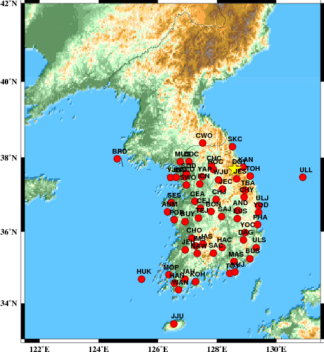
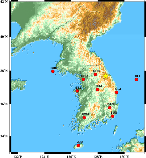
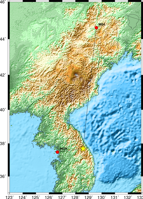
The focal mechanism was determined using accelerometer waveforms integrated to ground velocity. The location of the event and the station distribution are given in Figure 1.
|
|
|
      STK = 115
      DIP = 85
     RAKE = -5
       MW = 4.55
       HS = 9
The waveform inversion is preferred. This solution agrees with the surface-wave solution. This solution is well determined. Because of the size of this earthquake, waveform inversion was also performed using the accelereometer data converted to ground velocity. Care was taken to use the accelerometer traces only in the 0.05 - 0.2 Hz band, while the broadband sensor data were analyzed as usual in the 0.02 - 0.10 Hz band.
The program wvfgrd96 was used with good traces observed at short distance to determine the focal mechanism, depth and seismic moment. This technique requires a high quality signal and well determined velocity model for the Green functions. To the extent that these are the quality data, this type of mechanism should be preferred over the radiation pattern technique which requires the separate step of defining the pressure and tension quadrants and the correct strike.
The observed and predicted traces are filtered using the following gsac commands:
hp c 0.05 3
lp c 0.20 3
The results of this grid search from 0.5 to 19 km depth are as follow:
           DEPTH  STK   DIP  RAKE   MW    FIT
WVFGRD96    0.5   105    70   -25   4.22 0.3956
WVFGRD96    1.0   110    70   -20   4.24 0.4180
WVFGRD96    2.0   110    75   -20   4.30 0.4565
WVFGRD96    3.0   110    75   -15   4.35 0.5034
WVFGRD96    4.0   110    80   -20   4.40 0.5563
WVFGRD96    5.0   115    80   -15   4.45 0.6021
WVFGRD96    6.0   115    80   -10   4.48 0.6388
WVFGRD96    7.0   115    80   -10   4.51 0.6681
WVFGRD96    8.0   115    85   -10   4.54 0.6844
WVFGRD96    9.0   115    85    -5   4.55 0.6890
WVFGRD96   10.0   115    85    -5   4.57 0.6873
WVFGRD96   11.0   295    90     5   4.59 0.6862
WVFGRD96   12.0   115    90     0   4.60 0.6805
WVFGRD96   13.0   295    90     0   4.61 0.6751
WVFGRD96   14.0   295    85     0   4.62 0.6628
WVFGRD96   15.0   295    85    -5   4.62 0.6495
WVFGRD96   16.0   295    85    -5   4.63 0.6332
WVFGRD96   17.0   295    85    -5   4.64 0.6169
WVFGRD96   18.0   295    85    -5   4.65 0.6036
WVFGRD96   19.0   290    75   -10   4.64 0.5897
The best solution is
WVFGRD96 9.0 115 85 -5 4.55 0.6890
The mechanism correspond to the best fit is
|
|
|
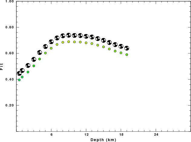
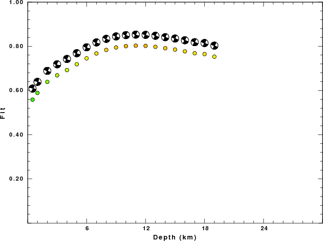
The best fit as a function of depth is given in the following figure:
|
|
|
The comparison of the observed and predicted waveforms is given in the next figure. The red traces are the observed and the blue are the predicted. Each observed-predicted componnet is plotted to the same scale and peak amplitudes are indicated by the numbers to the left of each trace. The number in black at the rightr of each predicted traces it the time shift required for maximum correlation between the observed and predicted traces. This time shift is required because the synthetics are not computed at exactly the same distance as the observed and because the velocity model used in the predictions may not be perfect. A positive time shift indicates that the prediction is too fast and should be delayed to match the observed trace (shift to the right in this figure). A negative value indicates that the prediction is too slow. The bandpass filter used in the processing and for the display was
hp c 0.05 3
lp c 0.20 3
|
|
|
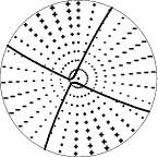
|
| Focal mechanism sensitivity at the preferred depth. The red color indicates a very good fit to thewavefroms. Each solution is plotted as a vector at a given value of strike and dip with the angle of the vector representing the rake angle, measured, with respect to the upward vertical (N) in the figure. |
|
|
|
The program wvfgrd96 was used with good traces observed at short distance to determine the focal mechanism, depth and seismic moment. This technique requires a high quality signal and well determined velocity model for the Green functions. To the extent that these are the quality data, this type of mechanism should be preferred over the radiation pattern technique which requires the separate step of defining the pressure and tension quadrants and the correct strike.
The observed and predicted traces are filtered using the following gsac commands:
hp c 0.02 3
lp c 0.10 3
The results of this grid search from 0.5 to 19 km depth are as follow:
           DEPTH  STK   DIP  RAKE   MW    FIT
WVFGRD96    0.5   290    80   -15   4.37 0.5586
WVFGRD96    1.0   290    85   -10   4.38 0.5890
WVFGRD96    2.0   295    90    -5   4.43 0.6387
WVFGRD96    3.0   110    75   -15   4.46 0.6684
WVFGRD96    4.0   115    75    -5   4.48 0.6925
WVFGRD96    5.0   115    80   -10   4.50 0.7186
WVFGRD96    6.0   115    80    -5   4.51 0.7454
WVFGRD96    7.0   115    80    -5   4.52 0.7674
WVFGRD96    8.0   115    85    -5   4.53 0.7835
WVFGRD96    9.0   115    85    -5   4.54 0.7946
WVFGRD96   10.0   115    85    -5   4.55 0.8005
WVFGRD96   11.0   115    85    -5   4.56 0.8027
WVFGRD96   12.0   115    85    -5   4.57 0.8017
WVFGRD96   13.0   115    90    -5   4.58 0.7975
WVFGRD96   14.0   295    90     5   4.58 0.7912
WVFGRD96   15.0   295    90     5   4.59 0.7851
WVFGRD96   16.0   115    90    -5   4.60 0.7771
WVFGRD96   17.0   115    90    -5   4.60 0.7685
WVFGRD96   18.0   115    85     5   4.61 0.7647
WVFGRD96   19.0   115    85     5   4.62 0.7529
The best solution is
WVFGRD96 11.0 115 85 -5 4.56 0.8027
The mechanism correspond to the best fit is

|
|
|
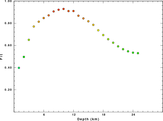
The best fit as a function of depth is given in the following figure:
|
|
|
The comparison of the observed and predicted waveforms is given in the next figure. The red traces are the observed and the blue are the predicted. Each observed-predicted componnet is plotted to the same scale and peak amplitudes are indicated by the numbers to the left of each trace. The number in black at the rightr of each predicted traces it the time shift required for maximum correlation between the observed and predicted traces. This time shift is required because the synthetics are not computed at exactly the same distance as the observed and because the velocity model used in the predictions may not be perfect. A positive time shift indicates that the prediction is too fast and should be delayed to match the observed trace (shift to the right in this figure). A negative value indicates that the prediction is too slow. The bandpass filter used in the processing and for the display was
hp c 0.02 3
lp c 0.10 3
|
|
|
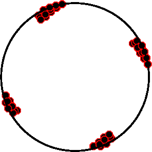
|
| Focal mechanism sensitivity at the preferred depth. The red color indicates a very good fit to thewavefroms. Each solution is plotted as a vector at a given value of strike and dip with the angle of the vector representing the rake angle, measured, with respect to the upward vertical (N) in the figure. |
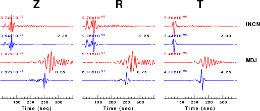
Broadband data for INCN and MDJ were obtained from the IRIS DMC. These waveform data were not inverted. Instead synthetics were generated using the preferred moment tensor solution given above. The ground velocity wasfiltered using the command
hp c 0.01 3
lp c 0.10 3
|
|
  NODAL PLANES


  STK=      25.00
  DIP=      90.00
 RAKE=     180.00

             OR

  STK=     115.00
  DIP=      90.00
 RAKE=       0.00


DEPTH = 10.0 km

Mw = 4.61
Best Fit 0.9289 - P-T axis plot gives solutions with FIT greater than FIT90
 |
|
The P-wave first motion plot using the Elocate location and take-off angles and the preferred focal mechanism is given here |
The P-wave first motion data for focal mechanism studies are as follow:
Sta Az(deg)    Dist(km)   First motion
DGY        91    7 iP_D
KAN        77   27 iP_D
JES       168   30 iP_C
TOH       114   51 iP_D
WJU       237   58 iP_D
HOC       269   63 iP_D
SKC       355   67 iP_C
CHC       278   69 iP_D
JEC       211   70 eP_C
TBA       153   71 iP_C
CHY       161   88 iP_C
YOJ       184   92 iP_C
YAP       257  100 iP_D
CHJ       211  106 iP_D
ICN       247  113 iP_D
CWO       310  122 iP_C
AND       175  124 iP_C
ULJ       146  131 iP_C
DDC       280  137 iP_D
SOD       265  144 eP_-
BON       209  145 eP_-
SAJ       195  148 iP_C
YOD       151  148 iP_C
EUS       177  149 iP_C
SEO       262  150 iP_D
SWO       252  152 iP_D
CEA       231  153 iP_D
CEJ       222  156 eP_X
MUS       278  163 eP_-
INC       263  176 iP_D
PHA       157  180 eP_+
TEJ       217  183 eP_-
YJD       263  193 eP_X
YOC       170  193 iP_C
ULL        96  205 iP_D
DAG       173  215 iP_C
SES       243  215 iP_D
BUY       224  217 eP_X
POR       231  237 eP_X
ANM       238  238 iP_C
HAC       189  240 iP_C
CHO       212  244 eP_X
JAS       203  245 eP_X
ULS       164  246 eP_X
IMS       207  259 eP_X
SAC       194  262 eP_+
BUS       170  275 eP_+
NAW       204  278 eP_X
MAS       180  280 iP_C
JEU       212  286 eP_X
KUJ       180  311 eP_X
TOY       183  316 eP_X
BRD       276  350 iP_D
KOH       200  362 eP_X
JAH       205  366 eP_X
MOP       213  377 eP_X
HAN       208  391 eP_X
WAN       206  404 eP_X
HUK       221  437 eP_-
JJU       202  508 eP_X
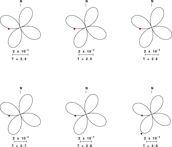
Surface wave analysis was performed using codes from Computer Programs in Seismology, specifically the multiple filter analysis program do_mft and the surface-wave radiation pattern search program srfgrd96.
Digital data were collected, instrument response removed and traces converted
to Z, R an T components. Multiple filter analysis was applied to the Z and T traces to obtain the Rayleigh- and Love-wave spectral amplitudes, respectively.
These were input to the search program which examined all depths between 1 and 25 km
and all possible mechanisms.
|
|
|
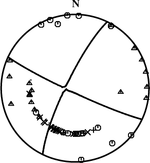
|
| Pressure-tension axis trends. Since the surface-wave spectra search does not distinguish between P and T axes and since there is a 180 ambiguity in strike, all possible P and T axes are plotted. First motion data and waveforms will be used to select the preferred mechanism. The purpose of this plot is to provide an idea of the possible range of solutions. The P and T-axes for all mechanisms with goodness of fit greater than 0.9 FITMAX (above) are plotted here. |
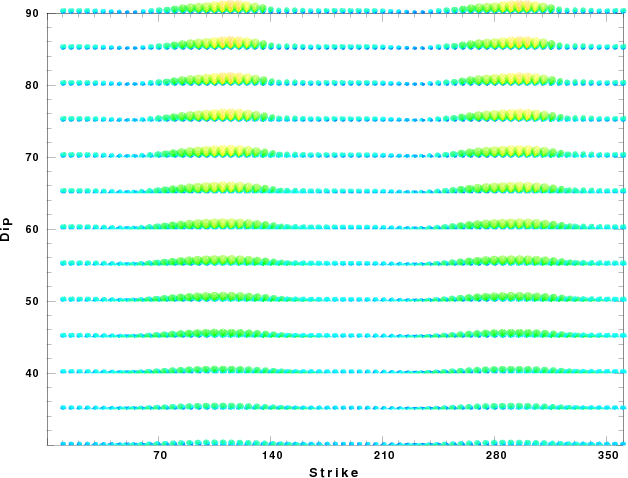
|
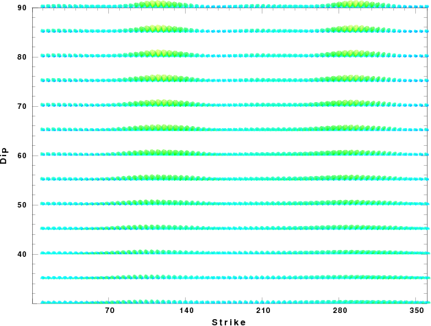
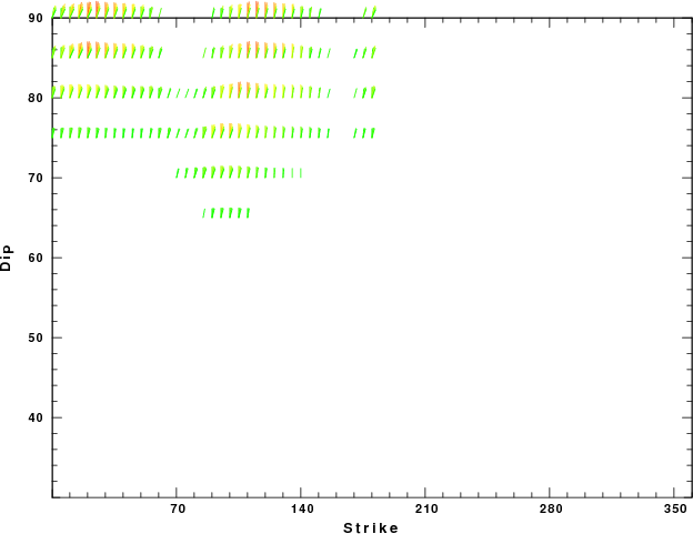
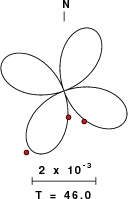
| Focal mechanism sensitivity at the preferred depth. The red color indicates a very good fit to the Love and Rayleigh wave radiation patterns. Each solution is plotted as a vector at a given value of strike and dip with the angle of the vector representing the rake angle, measured, with respect to the upward vertical (N) in the figure. Because of the symmetry of the spectral amplitude rediation patterns, only strikes from 0-180 degrees are sampled. |
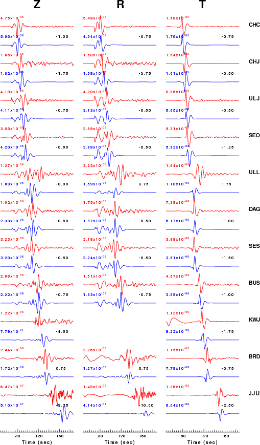
The distribution of broadband stations with azimuth and distance is
Sta Az(deg)    Dist(km)
CHC	  278	   69
CHJ	  211	  106
ULJ	  146	  131
SEO	  262	  150
INCN	  263	  174
DAG	  173	  215
SES	  243	  215
BUS	  170	  275
KWJ	  208	  316
BRD	  276	  350
JJU	  202	  508
Since the analysis of the surface-wave radiation patterns uses only spectral amplitudes and because the surfave-wave radiation patterns have a 180 degree symmetry, each surface-wave solution consists of four possible focal mechanisms corresponding to the interchange of the P- and T-axes and a roation of the mechanism by 180 degrees. To select one mechanism, P-wave first motion can be used. This was not possible in this case because all the P-wave first motions were emergent ( a feature of the P-wave wave takeoff angle, the station location and the mechanism). The other way to select among the mechanisms is to compute forward synthetics and compare the observed and predicted waveforms.
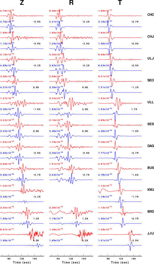
The fits to the waveforms with the given mechanism are show below:
|
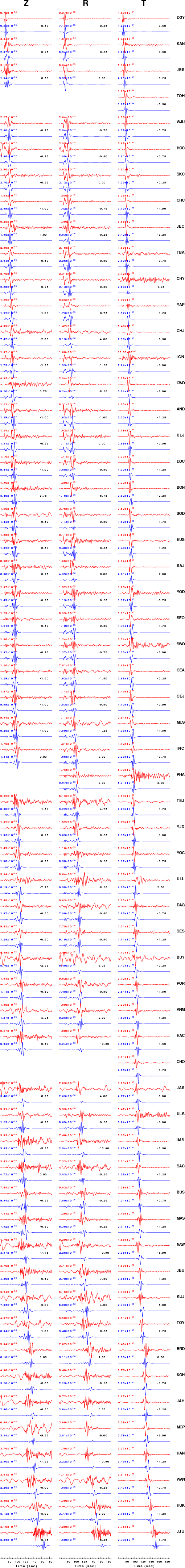
This figure shows the fit to the three components of motion (Z - vertical, R-radial and T - transverse). For each station and component, the observed traces is shown in red and the model predicted trace in blue. The traces represent filtered ground velocity in units of meters/sec (the peak value is printed adjacent to each trace; each pair of traces to plotted to the same scale to emphasize the difference in levels). Both synthetic and observed traces have been filtered using the SAC commands:
hp c 0.02 3
lp c 0.10 3
|
|
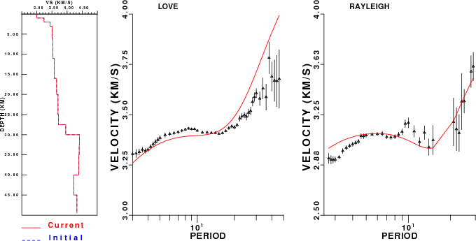
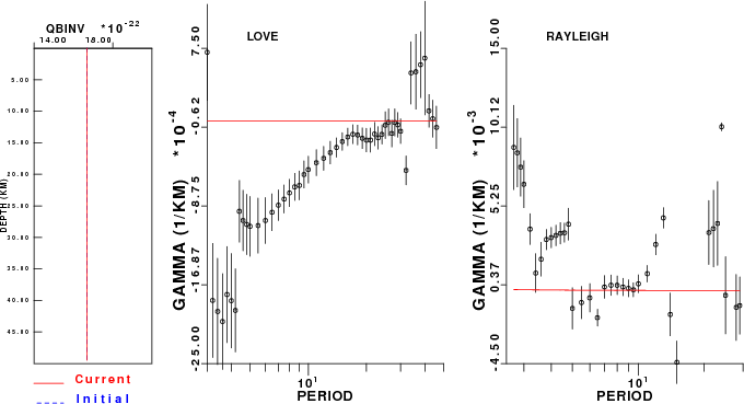
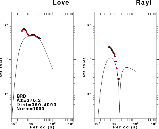
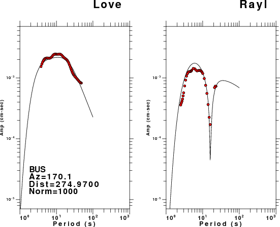
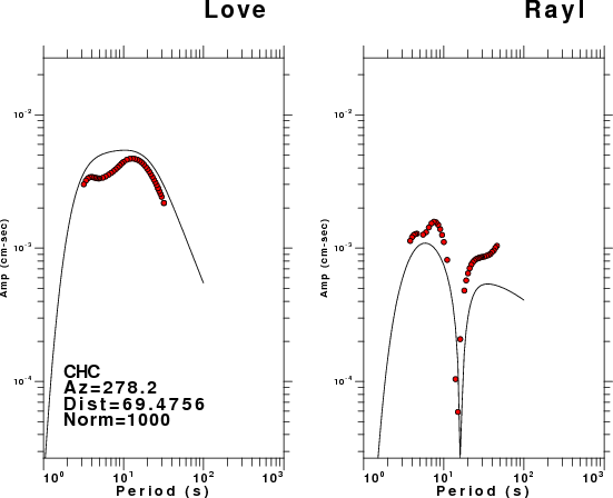
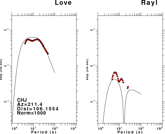
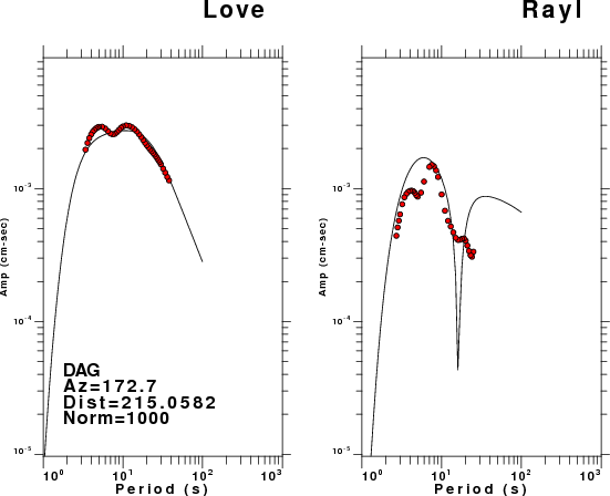
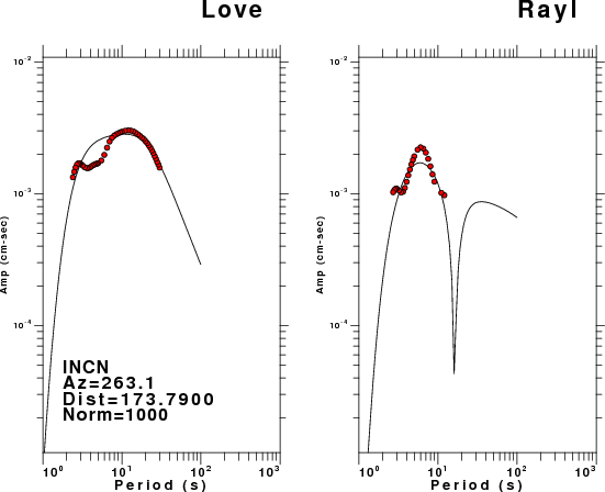
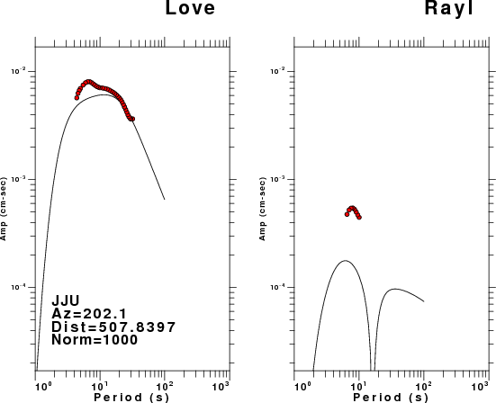
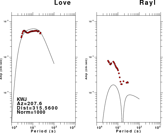
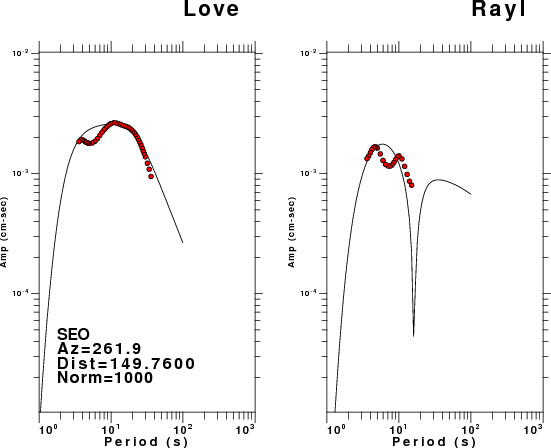
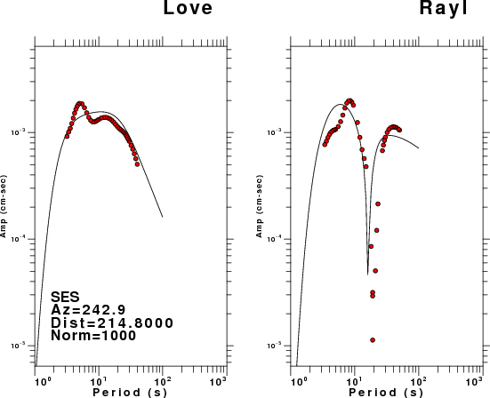
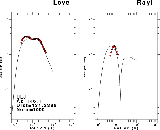
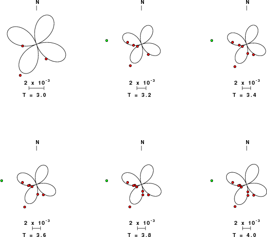
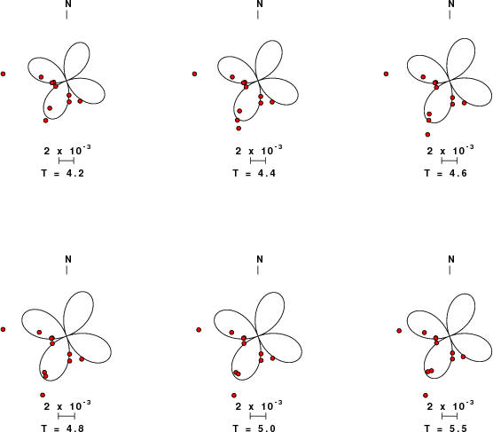
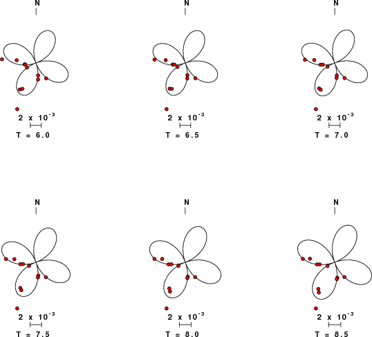
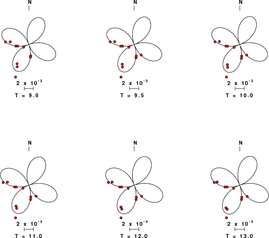
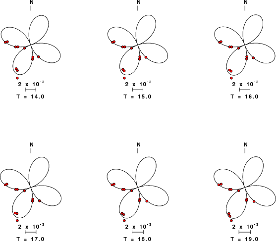
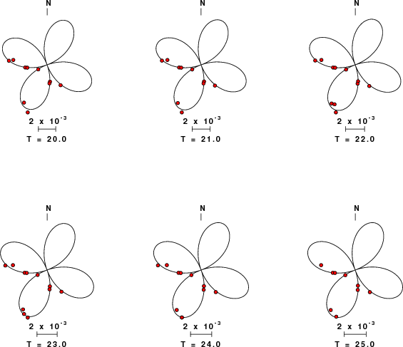
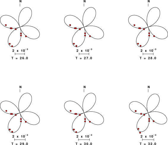
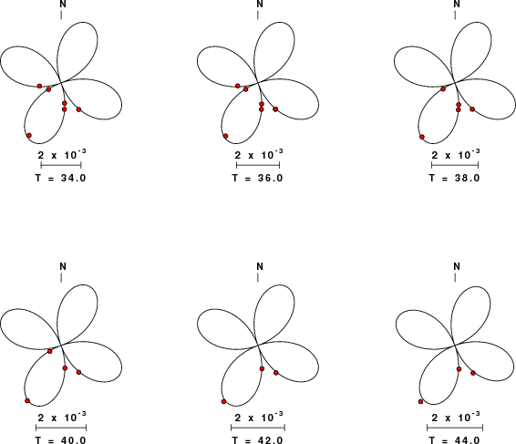
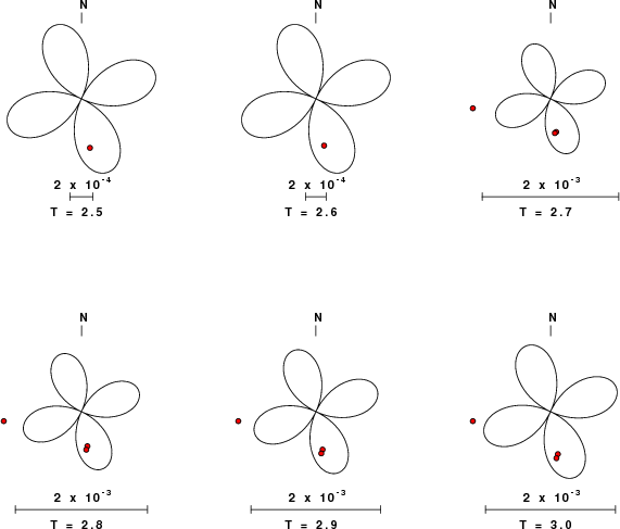
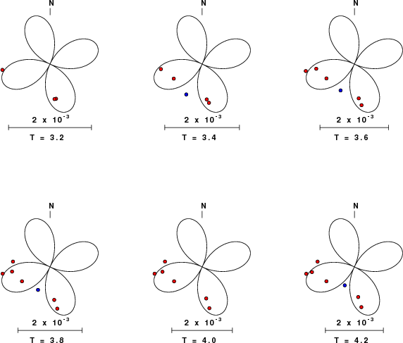
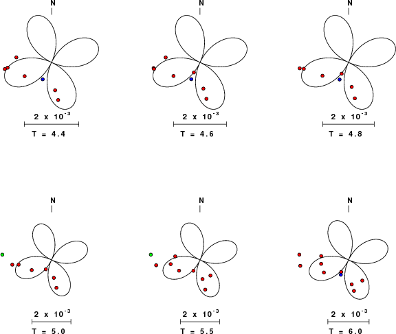
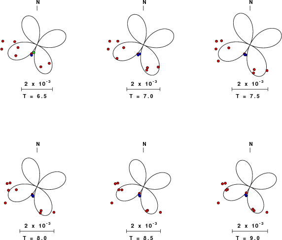
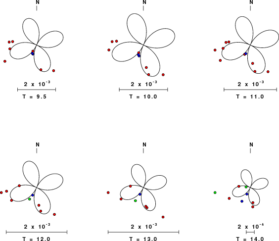
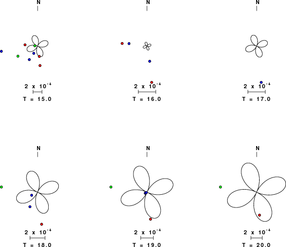
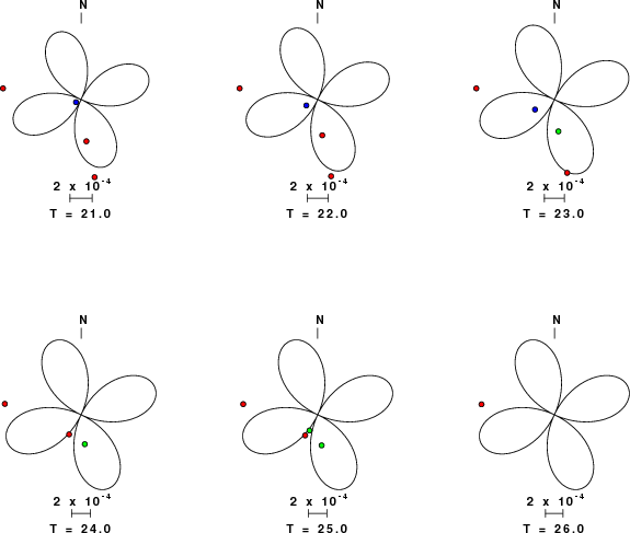
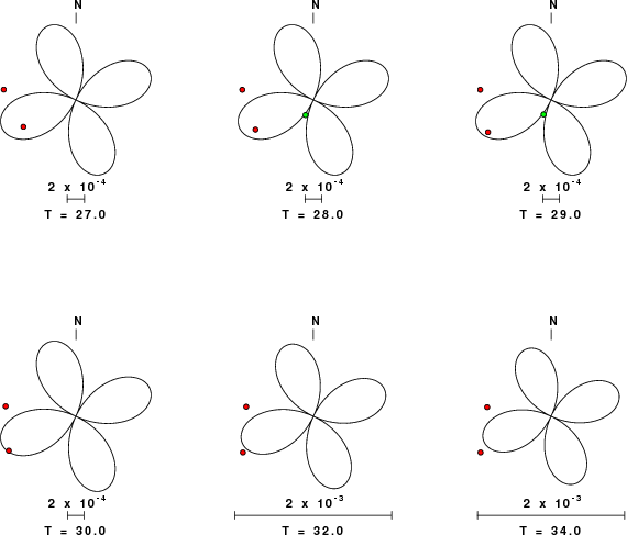
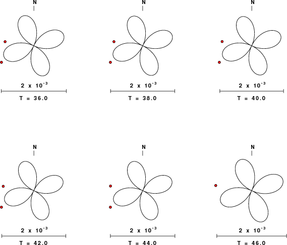
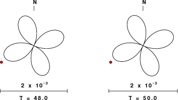
The figures below show the observed spectral amplitudes (units of cm-sec) at each station and the
theoretical predictions as a function of period for the mechanism given above. The modified Utah model earth model
was used to define the Green's functions. For each station, the Love and Rayleigh wave spectrail amplitudes are plotted with the same scaling so that one can get a sense fo the effects of the effects of the focal mechanism and depth on the excitation of each.
 |
 |
 |
 |
 |
 |
 |
 |
 |
 |
 |
Here we tabulate the reasons for not using certain digital data sets
PyeongChang's Olympic Bid Not Shaken by Tremor
Saturday’s moderate earthquake will not affect a bid by PyeongChang to host the 2014 Winter Olympics, a bid committee official said on Sunday.
PyeongChang, 150 kilometers east of Seoul, was cited as the epicenter of the quake that shook the country's eastern coastal region.
The tremor left some cracks in very old houses and buildings, but caused no damage to roads and other infrastructure,’’ Bang Jae-heung, secretary-general of the 2014 PyeongChang Olympic Winter Games Bid Committee, said.
Bang said the committee will make thorough preparations for the upcoming due diligence on its ability to host the games by the International Olympic Committee (IOC). The IOC inspections are scheduled for Feb. 14-17.
We hope that the earthquake will not create a bad image of PyeongChang. It was the first earthquake to affect the area, which has never been classified as earthquake-prone,’’ Bang said.
PyeongChang is vying to host the Winter Olympics and Paralympics along with two other contenders _ Salzburg, Austria, and Russia's Black Sea town of Sochi.
PyeongChang lost its bid for the 2010 Olympics to Vancouver, Canada, by only three votes. The final IOC vote on the 2014 Winter Olympics will take place in Guatemala in July.
If PyeongChang is successful, it would be the third Asian city to host the Winter Games. Two Japanese cities, Sapporo and Nagano, hosted the games in 1972 and 1998, respectively.