2004/05/29 10:14:24 36.67N 129.94E 11 5.08 Korea
 SLU Moment Tensor Solution
 2004/05/29 10:14:24 36.67N 129.94E 11 5.08 Korea

 Best Fitting Double Couple
    Mo = 4.68e+23 dyne-cm
    Mw = 5.08
    Z  = 11 km
     Plane   Strike  Dip  Rake
      NP1      193    62   101
      NP2      350    30    70
 Principal Axes:
   Axis    Value   Plunge  Azimuth
     T   4.68e+23     71     127
     N   0.00e+00     10       7
     P  -4.68e+23     16     275


 Moment Tensor: (dyne-cm)
    Component  Value
       Mxx     1.59e+22
       Mxy     1.01e+22
       Mxz    -9.83e+22
       Myy    -3.97e+23
       Myz     2.40e+23
       Mzz     3.81e+23


                     --------##----
                 ------------####------
              --------------#######-------
             -------------###########------
           --------------#############-------
          --------------################------
         --------------##################------
        --------------###################-------
        --------------####################------
       --   ---------#####################-------
       -- P ---------######################------
       --   ---------#########   ##########------
       -------------########## T ##########------
        ------------##########   ##########-----
        ------------######################------
         -----------######################-----
          ----------#####################-----
           ---------####################-----
             --------##################----
              -------#################----
                 -----##############---
                     --##########--


 Harvard Convention
 Moment Tensor:
      R          T          F
  3.81e+23  -9.83e+22  -2.40e+23
 -9.83e+22   1.59e+22  -1.01e+22
 -2.40e+23  -1.01e+22  -3.97e+23
|
USGS Fast Moment Tensor Solution

04/05/29 10:14:26.70
  SOUTH KOREA
  Epicenter:  36.670  129.944
  MW 5.3

  USGS MOMENT TENSOR SOLUTION
  Depth  17         No. of sta:  5
  Moment Tensor;   Scale 10**17 Nm
    Mrr= 0.65       Mtt= 0.32
    Mff=-0.97       Mrt=-0.54
    Mrf= 0.02       Mtf= 0.20
   Principal axes:
    T  Val=  1.05  Plg=53  Azm=175
    N       -0.04      37      347
    P       -1.01       4       80

  Best Double Couple:Mo=1.0*10**17
   NP1:Strike=202 Dip=52 Slip= 139
   NP2:       320     59        46


                #######
           #############----
         ############---------
       --------###--------------
     ------------#----------------
    -----------#####---------------
    ----------########------------
   ----------###########---------- P
   ----------############---------
   ---------###############---------
   --------#################--------
   --------##################-------
    -------########   #######------
    -------######## T ########-----
     ------########   ########----
       ----###################--
         ---##################
           --###############
                #######
|
Harvard CMT

 052904B SOUTH KOREA

  Date: 2004/ 5/29   Centroid Time: 10:14:30.0 GMT
  Lat=  36.71  Lon= 129.93
  Depth= 12.0   Half duration= 0.8
  Centroid time minus hypocenter time:  4.0
  Moment Tensor: Expo=23  4.500 0.110 -4.610 -0.560 1.440 0.410
  Mw = 5.1    mb = 5.3    Ms = 5.3   Scalar Moment = 4.83e+23
  Fault plane:  strike=180    dip=36   slip=99
  Fault plane:  strike=350    dip=54   slip=84
|
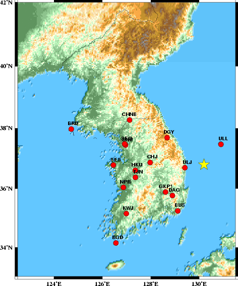
The focal mechanism was determined using broadband seismic waveforms. The location of the event and the station distribution are given in Figure 1.
|
|
|
|
      STK = 350
      DIP = 30
     RAKE = 70
       MW = 5.08
       HS = 11
The waveform inversion is preferred. This solution agrees with the surfac-ewave solution. This solution is well determined.
The program wvfgrd96 was used with good traces observed at short distance to determine the focal mechanism, depth and seismic moment. This technique requires a high quality signal and well determined velocity model for the Green functions. To the extent that these are the quality data, this type of mechanism should be preferred over the radiation pattern technique which requires the separate step of defining the pressure and tension quadrants and the correct strike.
The observed and predicted traces are filtered using the following gsac commands:
hp c 0.02 3
lp c 0.10 3
The results of this grid search from 0.5 to 19 km depth are as follow:
           DEPTH  STK   DIP  RAKE   MW    FIT
WVFGRD96    0.5   185    60   -90   4.91 0.4884
WVFGRD96    1.0   185    55   -85   4.93 0.4869
WVFGRD96    2.0   185    65   -85   5.00 0.4220
WVFGRD96    3.0   300    20    15   5.00 0.4414
WVFGRD96    4.0   300    20    20   5.00 0.4938
WVFGRD96    5.0   305    20    25   4.99 0.5356
WVFGRD96    6.0   315    20    40   5.00 0.5696
WVFGRD96    7.0   355    20    75   5.02 0.5960
WVFGRD96    8.0   355    20    75   5.03 0.6176
WVFGRD96    9.0   355    25    75   5.05 0.6329
WVFGRD96   10.0   350    25    70   5.06 0.6411
WVFGRD96   11.0   350    30    70   5.08 0.6438
WVFGRD96   12.0   350    30    70   5.09 0.6435
WVFGRD96   13.0   355    35    80   5.09 0.6399
WVFGRD96   14.0   355    40    80   5.10 0.6338
WVFGRD96   15.0   355    40    80   5.11 0.6263
WVFGRD96   16.0   360    45    85   5.11 0.6129
WVFGRD96   17.0   360    45    85   5.13 0.6022
WVFGRD96   18.0   355    45    80   5.13 0.5862
WVFGRD96   19.0   180    40    90   5.13 0.5688
WVFGRD96   20.0   360    50    90   5.14 0.5479
WVFGRD96   21.0   180    40    90   5.14 0.5246
WVFGRD96   22.0   180    35    85   5.15 0.4995
WVFGRD96   23.0   180    35    85   5.15 0.4737
WVFGRD96   24.0   180    35    85   5.15 0.4467
WVFGRD96   25.0   180    35    85   5.16 0.4185
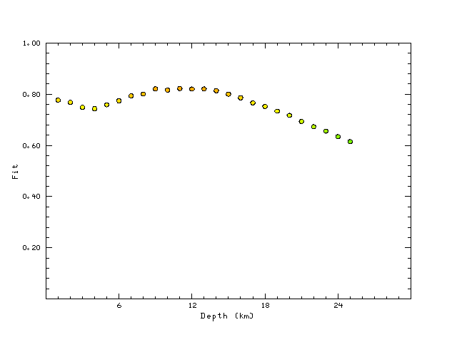
The best solution is
WVFGRD96 11.0 350 30 70 5.08 0.6438
The mechanism correspond to the best fit is
|
|
|
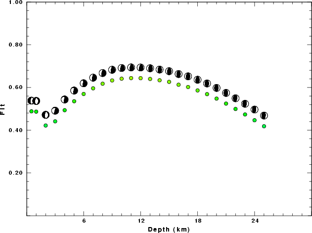
The best fit as a function of depth is given in the following figure:
|
|
|
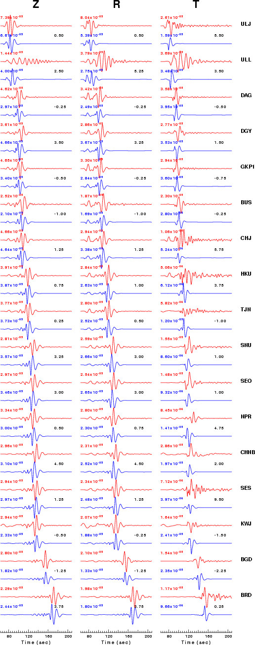
The comparison of the observed and predicted waveforms is given in the next figure. The red traces are the observed and the blue are the predicted. Each observed-predicted componnet is plotted to the same scale and peak amplitudes are indicated by the numbers to the left of each trace. The number in black at the rightr of each predicted traces it the time shift required for maximum correlation between the observed and predicted traces. This time shift is required because the synthetics are not computed at exactly the same distance as the observed and because the velocity model used in the predictions may not be perfect. A positive time shift indicates that the prediction is too fast and should be delayed to match the observed trace (shift to the right in this figure). A negative value indicates that the prediction is too slow. The bandpass filter used in the processing and for the display was
hp c 0.02 3
lp c 0.10 3
|
|
|
|
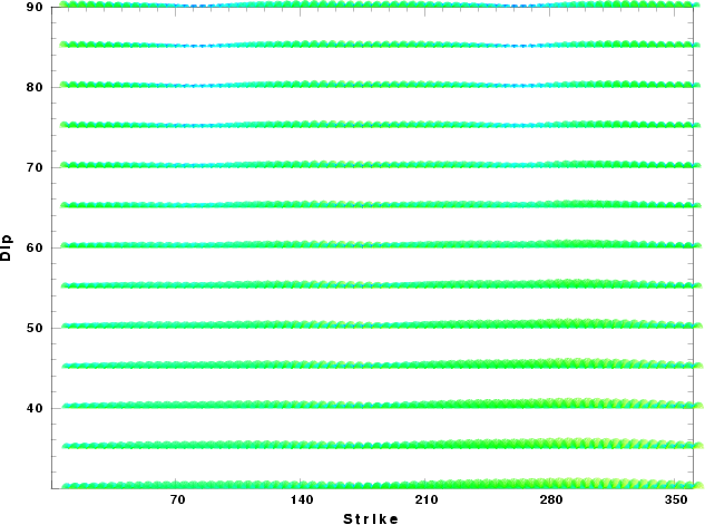
| Focal mechanism sensitivity at the preferred depth. The red color indicates a very good fit to thewavefroms. Each solution is plotted as a vector at a given value of strike and dip with the angle of the vector representing the rake angle, measured, with respect to the upward vertical (N) in the figure. |
  NODAL PLANES


  STK=     185.00
  DIP=      50.00
 RAKE=      90.00

             OR

  STK=       5.00
  DIP=      40.00
 RAKE=      90.00


DEPTH = 11.0 km

Mw = 5.10
Best Fit 0.8222 - P-T axis plot gives solutions with FIT greater than FIT90
 |
The P-wave first motion data for focal mechanism studies are as follow:
Sta Az(deg)    Dist(km)   First motion
ULJ       261   72 iP_D
ULL        40   97 iP_D
DAG       226  164 iP_C
DGY       307  168 iP_C
GKP1      235  175 iP_C
BUS       210  198 iP_C
CHJ       273  199 iP_C
HKU       266  255 iP_C
TJN       260  258 iP_C
SNU       285  297 eP_+
SEO       286  301 eP_+
NPR       255  310 iP_C
CHNB      302  317 iP_C
SES       271  334 iP_C
KWJ       239  342 iP_C
BGD       229  442 eP_+
BRD       286  510 eP_+
Surface wave analysis was performed using codes from Computer Programs in Seismology, specifically the multiple filter analysis program do_mft and the surface-wave radiation pattern search program srfgrd96.
Digital data were collected, instrument response removed and traces converted
to Z, R an T components. Multiple filter analysis was applied to the Z and T traces to obtain the Rayleigh- and Love-wave spectral amplitudes, respectively.
These were input to the search program which examined all depths between 1 and 25 km
and all possible mechanisms.
|
|
|

|
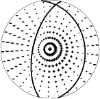
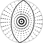
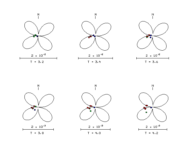
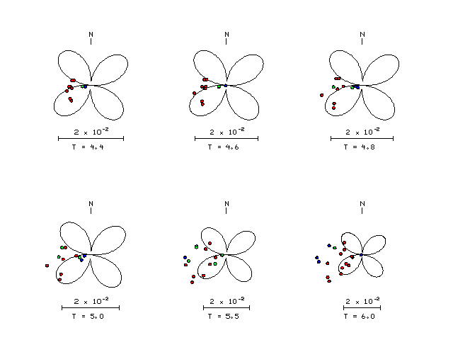
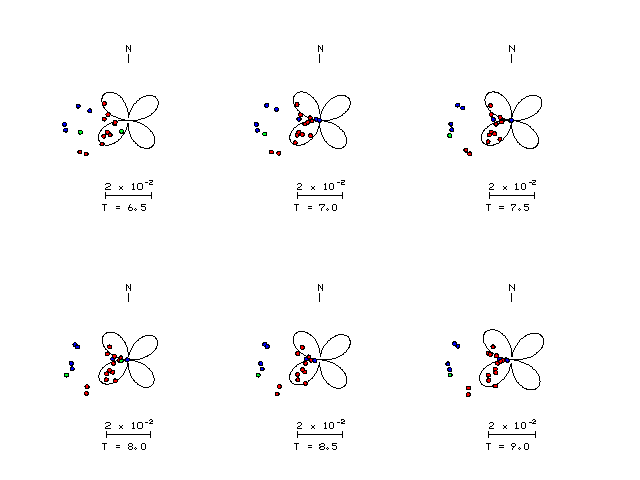
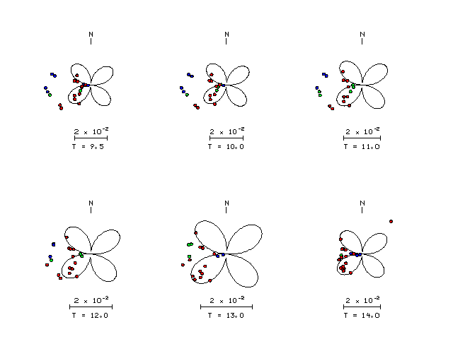
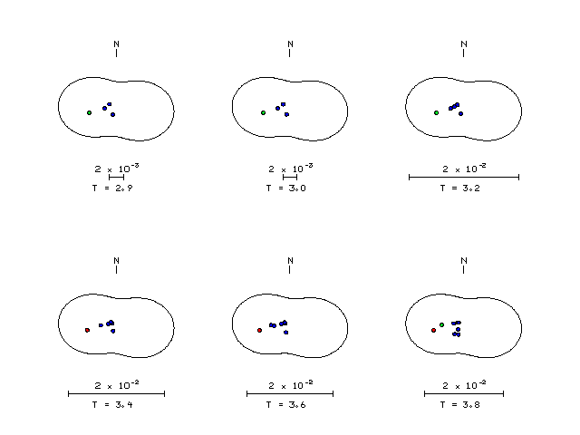
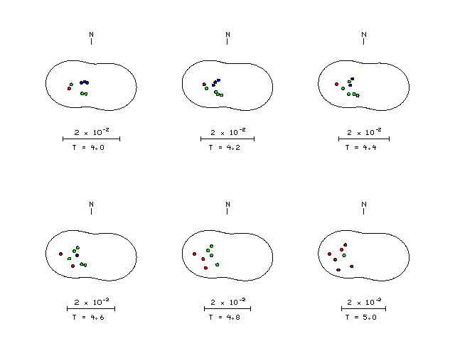
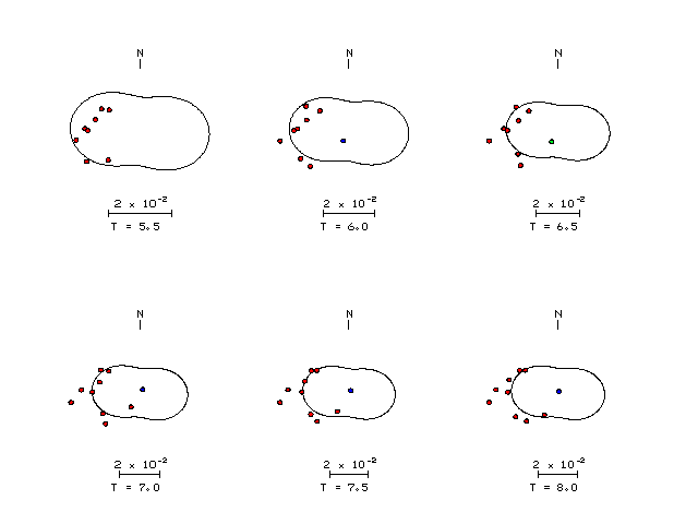
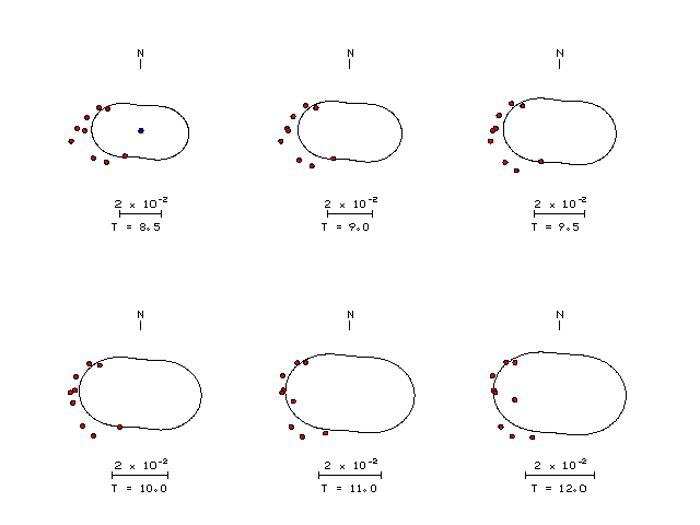
| Pressure-tension axis trends. Since the surface-wave spectra search does not distinguish between P and T axes and since there is a 180 ambiguity in strike, all possible P and T axes are plotted. First motion data and waveforms will be used to select the preferred mechanism. The purpose of this plot is to provide an idea of the possible range of solutions. The P and T-axes for all mechanisms with goodness of fit greater than 0.9 FITMAX (above) are plotted here. |
|
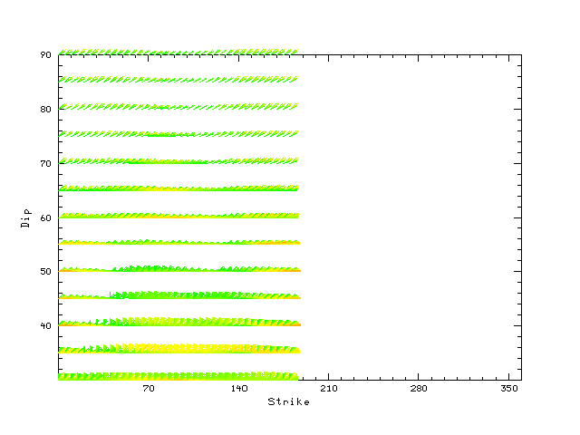
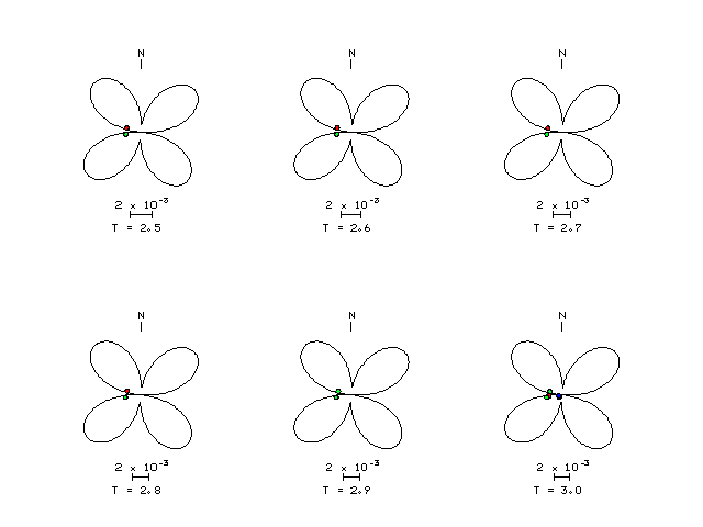
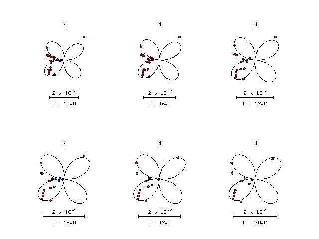
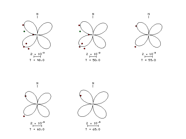
| Focal mechanism sensitivity at the preferred depth. The red color indicates a very good fit to the Love and Rayleigh wave radiation patterns. Each solution is plotted as a vector at a given value of strike and dip with the angle of the vector representing the rake angle, measured, with respect to the upward vertical (N) in the figure. Because of the symmetry of the spectral amplitude rediation patterns, only strikes from 0-180 degrees are sampled. |
The distribution of broadband stations with azimuth and distance is
Sta Az(deg)    Dist(km)
ULJ	  262	   72
ULL	   40	   97
DAG	  226	  164
DGY	  307	  168
GKP1	  235	  175
BUS	  210	  198
CHJ	  273	  199
HKU	  266	  255
TJN	  260	  258
SNU	  285	  297
SEO	  286	  301
NPR	  255	  310
CHNB	  302	  317
SES	  271	  334
KWJ	  239	  342
BGD	  230	  442
BRD	  287	  503
Since the analysis of the surface-wave radiation patterns uses only spectral amplitudes and because the surfave-wave radiation patterns have a 180 degree symmetry, each surface-wave solution consists of four possible focal mechanisms corresponding to the interchange of the P- and T-axes and a roation of the mechanism by 180 degrees. To select one mechanism, P-wave first motion can be used. This was not possible in this case because all the P-wave first motions were emergent ( a feature of the P-wave wave takeoff angle, the station location and the mechanism). The other way to select among the mechanisms is to compute forward synthetics and compare the observed and predicted waveforms.
The fits to the waveforms with the given mechanism are show below:
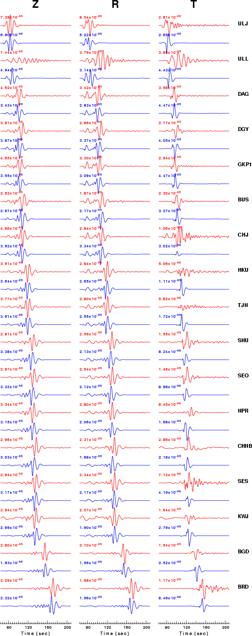
|
This figure shows the fit to the three components of motion (Z - vertical, R-radial and T - transverse). For each station and component, the observed traces is shown in red and the model predicted trace in blue. The traces represent filtered ground velocity in units of meters/sec (the peak value is printed adjacent to each trace; each pair of traces to plotted to the same scale to emphasize the difference in levels). Both synthetic and observed traces have been filtered using the SAC commands:
hp c 0.02 3
lp c 0.10 3
|
|
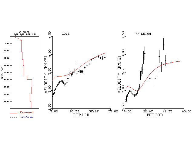
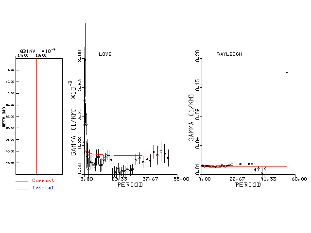
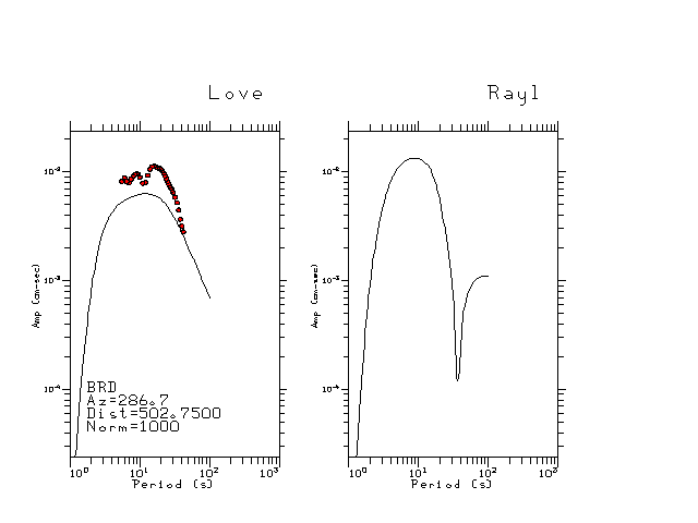
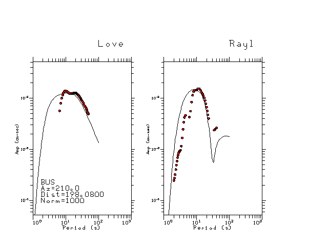
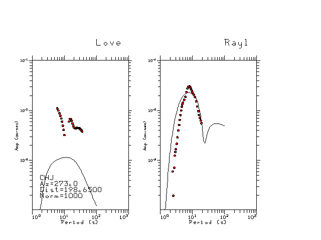
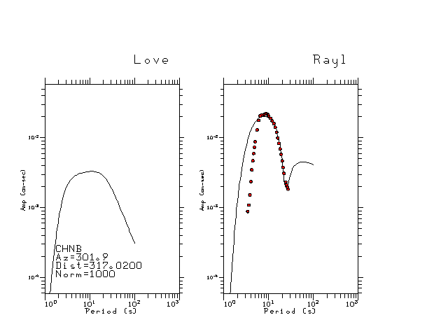
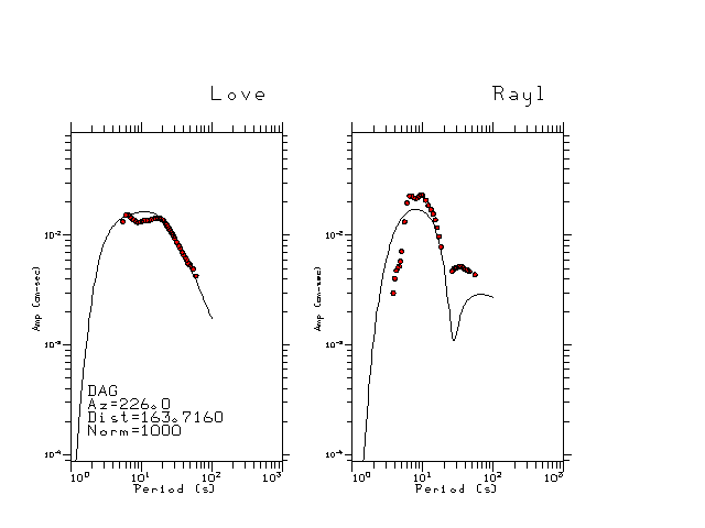
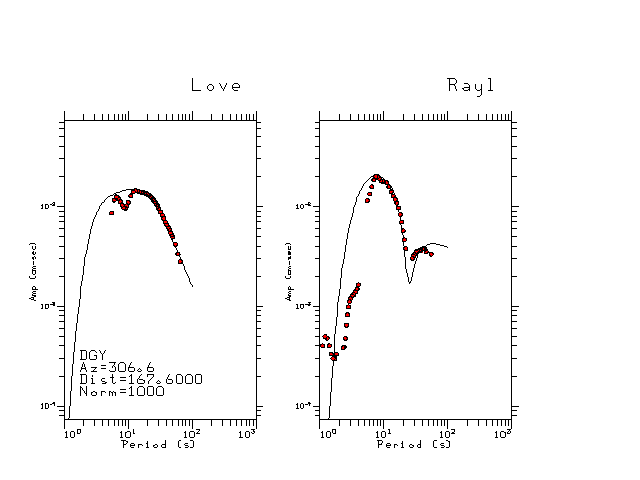
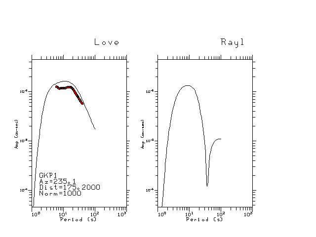
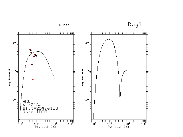
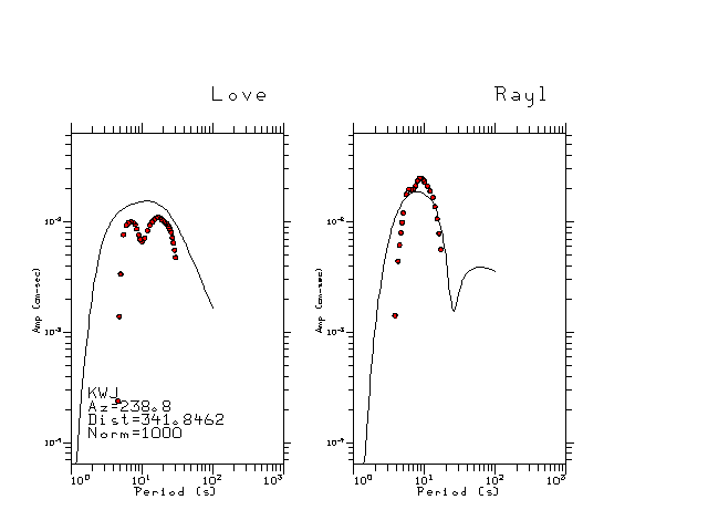
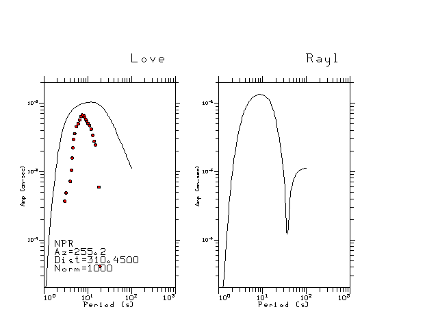
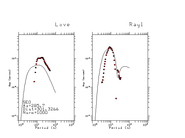
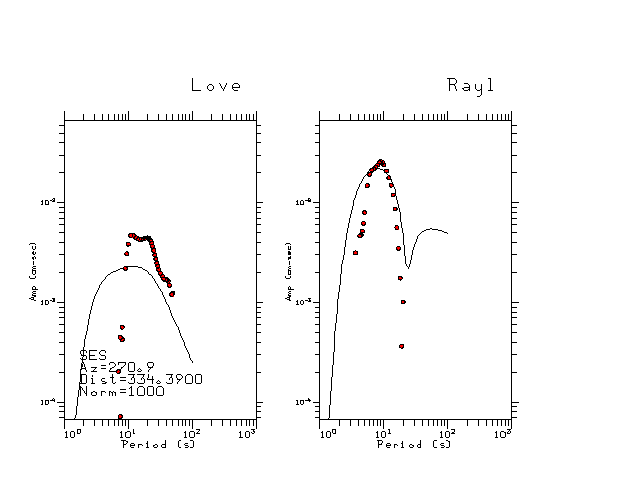
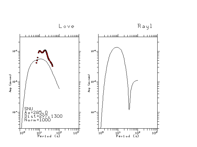
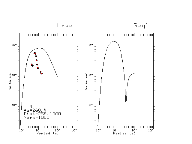
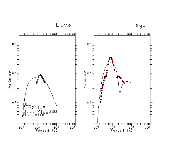
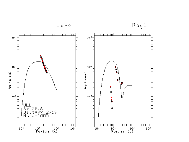
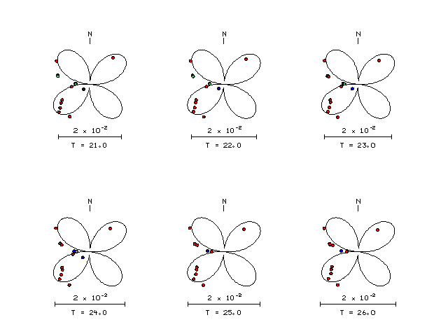
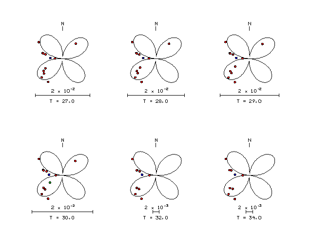
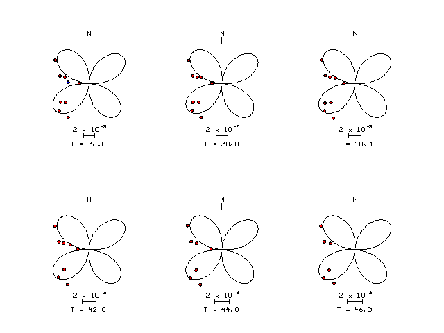
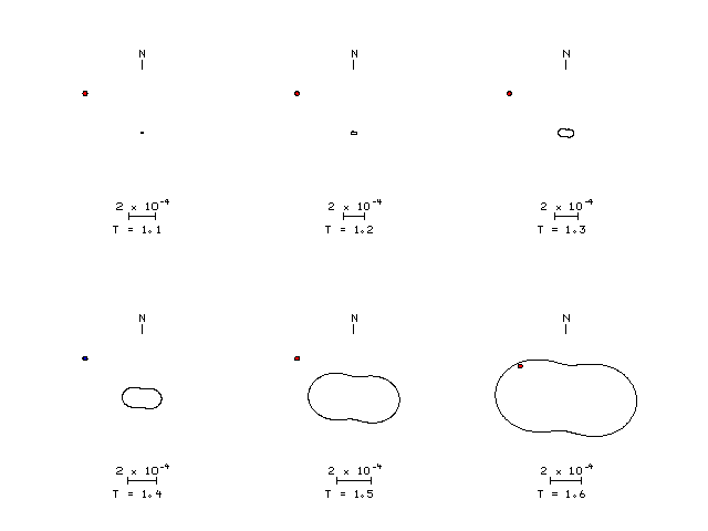
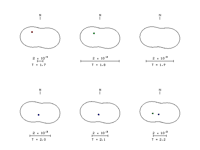
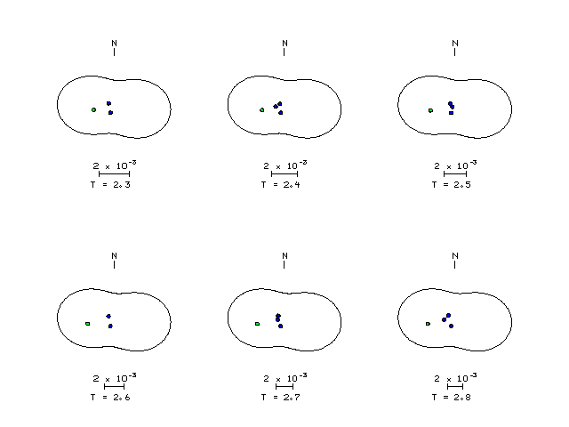
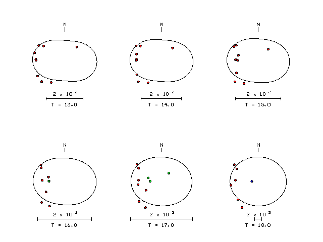
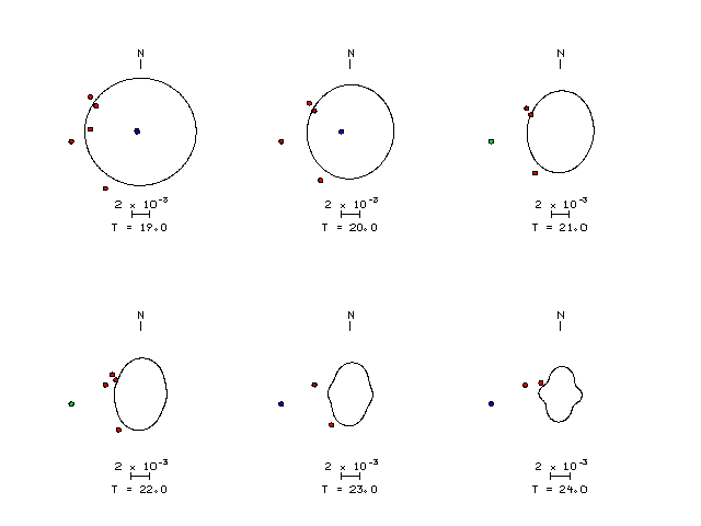
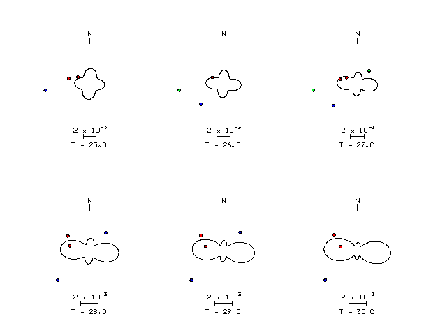
The figures below show the observed spectral amplitudes (units of cm-sec) at each station and the
theoretical predictions as a function of period for the mechanism given above. The modified Utah model earth model
was used to define the Green's functions. For each station, the Love and Rayleigh wave spectrail amplitudes are plotted with the same scaling so that one can get a sense fo the effects of the effects of the focal mechanism and depth on the excitation of each.
 |
 |
 |
 |
 |
 |
 |
 |
 |
 |
 |
 |
 |
 |
 |
 |
 |
Here we tabulate the reasons for not using certain digital data sets