2002/07/23 12:48:04 35.57N 122.18E 9 4.80 Korea
 SLU Moment Tensor Solution
 2002/07/23 12:48:04 35.57N 122.18E 9 4.80 Korea

 Best Fitting Double Couple
    Mo = 2.19e+23 dyne-cm
    Mw = 4.86
    Z  = 17 km
     Plane   Strike  Dip  Rake
      NP1      202    81   -20
      NP2      295    70   -170
 Principal Axes:
   Axis    Value   Plunge  Azimuth
     T   2.19e+23      7     250
     N   0.00e+00     68     358
     P  -2.19e+23     21     157


 Moment Tensor: (dyne-cm)
    Component  Value
       Mxx    -1.35e+23
       Mxy     1.39e+23
       Mxz     5.75e+22
       Myy     1.59e+23
       Myz    -5.45e+22
       Mzz    -2.44e+22


                     --------------
                 -----------------#####
              -------------------#########
             -------------------###########
           --------------------##############
          --------------------################
         ##########----------##################
        ##################--####################
        ###################---##################
       ####################-------###############
       ###################-----------############
       ##################--------------##########
       #################------------------#######
           #############--------------------####
         T ############----------------------###
           ############------------------------
          ############------------------------
           ###########-----------------------
             ########------------   -------
              #######------------ P ------
                 ####------------   ---
                     --------------


 Harvard Convention
 Moment Tensor:
      R          T          F
 -2.44e+22   5.75e+22   5.45e+22
  5.75e+22  -1.35e+23  -1.39e+23
  5.45e+22  -1.39e+23   1.59e+23
|
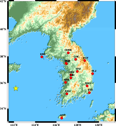
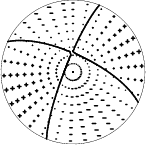
The focal mechanism was determined using broadband seismic waveforms. The location of the event and the station distribution are given in Figure 1.
|
|
|
|
      STK = 295
      DIP = 70
     RAKE = -170
       MW = 4.86
       HS = 17
This is not a well determined mechanism. The moment is well constrained, but the mechanism is not. The surface-wave inversion is preferred. This was difficult to model because of the high frequency coda following the surface wave - hence the relatively low frequency bandpass filter corner. The P-wave first motions were marginal and of no assistance in determining the solutions. The crossing nodal planes in the NE quadrant would give low P-wave amplitudes to Korea. The Love wave radiation pattern data are superb.
The program wvfgrd96 was used with good traces observed at short distance to determine the focal mechanism, depth and seismic moment. This technique requires a high quality signal and well determined velocity model for the Green functions. To the extent that these are the quality data, this type of mechanism should be preferred over the radiation pattern technique which requires the separate step of defining the pressure and tension quadrants and the correct strike.
The observed and predicted traces are filtered using the following gsac commands:
hp c 0.01 4
lp c 0.06 4
The results of this grid search from 0.5 to 19 km depth are as follow:
           DEPTH  STK   DIP  RAKE   MW    FIT
WVFGRD96    0.5   205    75    35   4.66 0.3981
WVFGRD96    1.0   195    85     5   4.59 0.4230
WVFGRD96    2.0    20    90     0   4.63 0.4472
WVFGRD96    3.0    20    85     5   4.66 0.4677
WVFGRD96    4.0    25    80    20   4.72 0.4873
WVFGRD96    5.0   200    85   -25   4.74 0.5121
WVFGRD96    6.0   200    85   -30   4.76 0.5312
WVFGRD96    7.0   200    85   -30   4.77 0.5448
WVFGRD96    8.0   200    80   -30   4.79 0.5554
WVFGRD96    9.0   200    80   -30   4.79 0.5615
WVFGRD96   10.0   200    80   -25   4.80 0.5653
WVFGRD96   11.0   200    80   -25   4.80 0.5670
WVFGRD96   12.0   200    80   -25   4.80 0.5639
WVFGRD96   13.0   200    85   -20   4.80 0.5607
WVFGRD96   14.0   200    85   -20   4.81 0.5572
WVFGRD96   15.0   200    85   -20   4.81 0.5555
WVFGRD96   16.0   200    85   -20   4.81 0.5518
WVFGRD96   17.0   200    85   -20   4.82 0.5459
WVFGRD96   18.0   200    85   -20   4.82 0.5429
WVFGRD96   19.0   200    85   -20   4.83 0.5384
WVFGRD96   20.0   200    85   -20   4.84 0.5357
WVFGRD96   21.0   200    85   -20   4.84 0.5323
WVFGRD96   22.0   200    85   -15   4.86 0.5291
WVFGRD96   23.0   200    85   -15   4.87 0.5280
WVFGRD96   24.0   200    85   -15   4.88 0.5278
WVFGRD96   25.0   200    80   -15   4.89 0.5283
The best solution is
WVFGRD96 11.0 200 80 -25 4.80 0.5670
The mechanism correspond to the best fit is
|
|
|
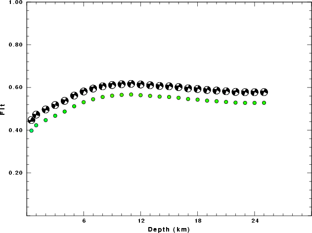
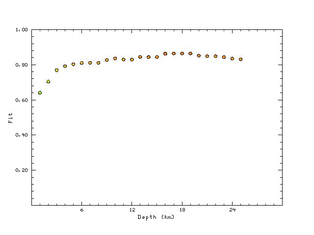
The best fit as a function of depth is given in the following figure:
|
|
|
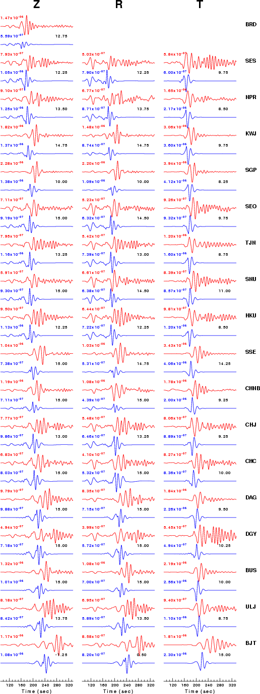
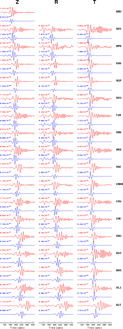
The comparison of the observed and predicted waveforms is given in the next figure. The red traces are the observed and the blue are the predicted. Each observed-predicted componnet is plotted to the same scale and peak amplitudes are indicated by the numbers to the left of each trace. The number in black at the rightr of each predicted traces it the time shift required for maximum correlation between the observed and predicted traces. This time shift is required because the synthetics are not computed at exactly the same distance as the observed and because the velocity model used in the predictions may not be perfect. A positive time shift indicates that the prediction is too fast and should be delayed to match the observed trace (shift to the right in this figure). A negative value indicates that the prediction is too slow. The bandpass filter used in the processing and for the display was
hp c 0.01 4
lp c 0.06 4
|
|
|
|
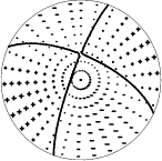
| Focal mechanism sensitivity at the preferred depth. The red color indicates a very good fit to thewavefroms. Each solution is plotted as a vector at a given value of strike and dip with the angle of the vector representing the rake angle, measured, with respect to the upward vertical (N) in the figure. |
  NODAL PLANES


  STK=     201.53
  DIP=      80.60
 RAKE=     -20.28

             OR

  STK=     294.98
  DIP=      70.00
 RAKE=    -169.99


DEPTH = 18.0 km

Mw = 4.80
Best Fit 0.8644 - P-T axis plot gives solutions with FIT greater than FIT90
 |
The P-wave first motion data for focal mechanism studies are as follow:
Sta Az(deg)    Dist(km)   First motion
BRD        39  344 eP_X
SES        69  407 eP_-
NPR        82  427 eP_+
KWJ        95  440 eP_+
SGP       122  473 eP_X
SEO        62  475 eP_-
SNU        63  476 eP_X
TJN        78  476 eP_+
HKU        75  481 eP_X
SSE       191  505 iP_+
CHNB       54  533 eP_-
CHJ        73  541 eP_+
CHC        62  560 eP_-
DAG        86  608 eP_+
DGY        66  627 eP_X
BUS        91  631 eP_X
ULJ        77  662 eP_-
BJT       315  724 eP_X
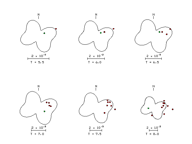
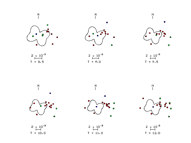
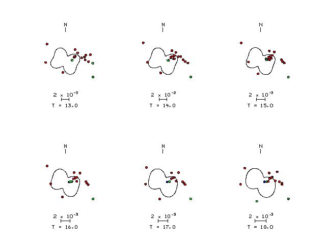
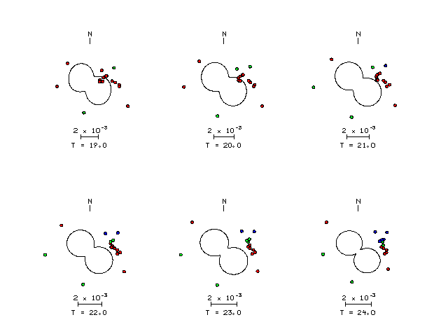
Surface wave analysis was performed using codes from Computer Programs in Seismology, specifically the multiple filter analysis program do_mft and the surface-wave radiation pattern search program srfgrd96.
Digital data were collected, instrument response removed and traces converted
to Z, R an T components. Multiple filter analysis was applied to the Z and T traces to obtain the Rayleigh- and Love-wave spectral amplitudes, respectively.
These were input to the search program which examined all depths between 1 and 25 km
and all possible mechanisms.
|
|
|
|
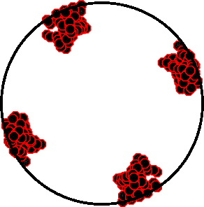
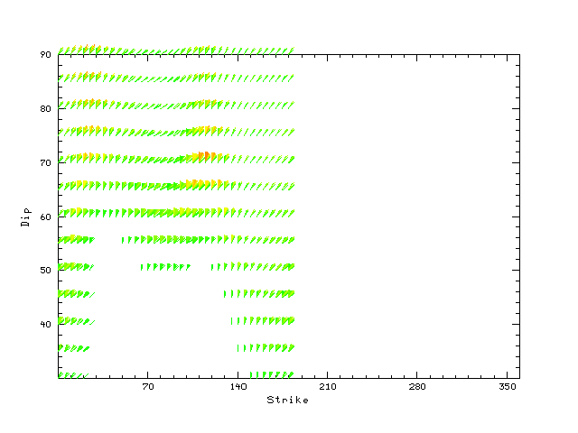
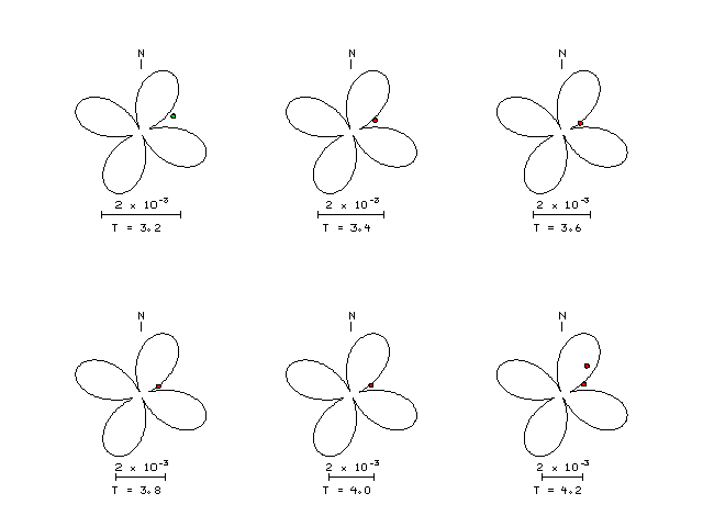
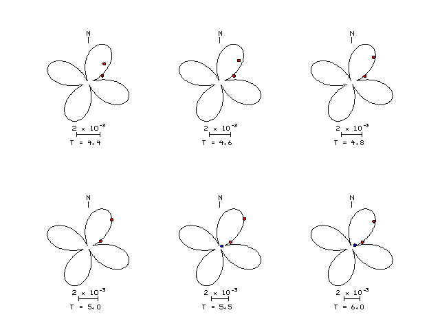
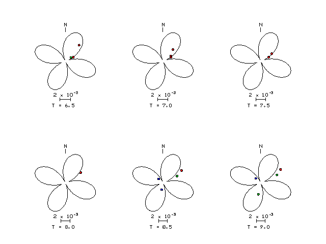
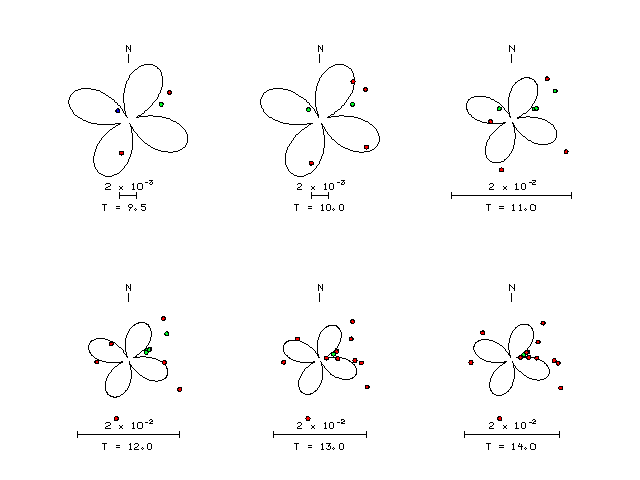
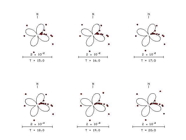
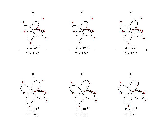
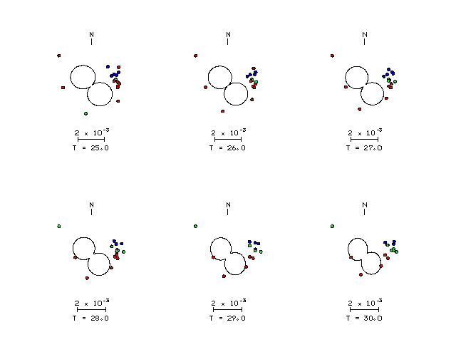
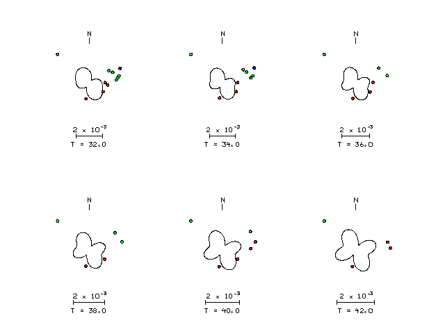
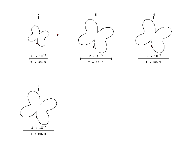
| Pressure-tension axis trends. Since the surface-wave spectra search does not distinguish between P and T axes and since there is a 180 ambiguity in strike, all possible P and T axes are plotted. First motion data and waveforms will be used to select the preferred mechanism. The purpose of this plot is to provide an idea of the possible range of solutions. The P and T-axes for all mechanisms with goodness of fit greater than 0.9 FITMAX (above) are plotted here. |
|
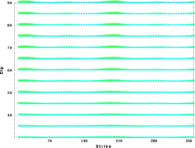
| Focal mechanism sensitivity at the preferred depth. The red color indicates a very good fit to the Love and Rayleigh wave radiation patterns. Each solution is plotted as a vector at a given value of strike and dip with the angle of the vector representing the rake angle, measured, with respect to the upward vertical (N) in the figure. Because of the symmetry of the spectral amplitude rediation patterns, only strikes from 0-180 degrees are sampled. |
The distribution of broadband stations with azimuth and distance is
Sta Az(deg)    Dist(km)
BRD	   39	  344
NPR	   82	  427
KWJ	   95	  440
SGP	  122	  473
SEO	   62	  475
SNU	   63	  476
TJN	   78	  476
HKU	   75	  481
SSE	  191	  505
CHNB	   54	  532
CHJ	   73	  541
CHC	   62	  560
DAG	   86	  608
DGY	   66	  627
BUS	   91	  631
ULJ	   77	  662
BJT	  315	  724
XAN	  266	 1224
Since the analysis of the surface-wave radiation patterns uses only spectral amplitudes and because the surfave-wave radiation patterns have a 180 degree symmetry, each surface-wave solution consists of four possible focal mechanisms corresponding to the interchange of the P- and T-axes and a roation of the mechanism by 180 degrees. To select one mechanism, P-wave first motion can be used. This was not possible in this case because all the P-wave first motions were emergent ( a feature of the P-wave wave takeoff angle, the station location and the mechanism). The other way to select among the mechanisms is to compute forward synthetics and compare the observed and predicted waveforms.
The fits to the waveforms with the given mechanism are show below:
|
This figure shows the fit to the three components of motion (Z - vertical, R-radial and T - transverse). For each station and component, the observed traces is shown in red and the model predicted trace in blue. The traces represent filtered ground velocity in units of meters/sec (the peak value is printed adjacent to each trace; each pair of traces to plotted to the same scale to emphasize the difference in levels). Both synthetic and observed traces have been filtered using the SAC commands:
hp c 0.01 4
lp c 0.06 4
|
|
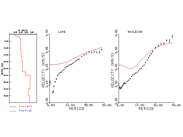
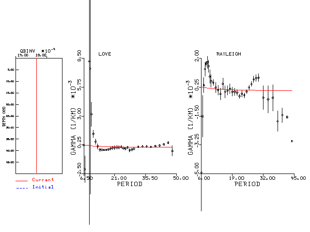
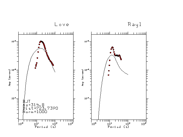
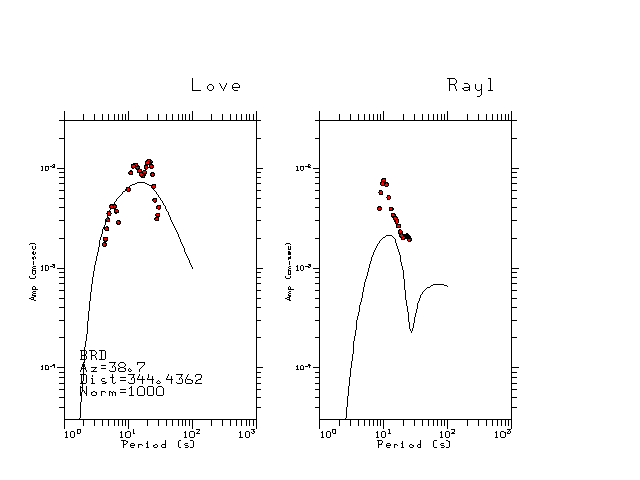
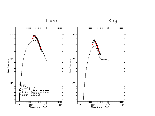
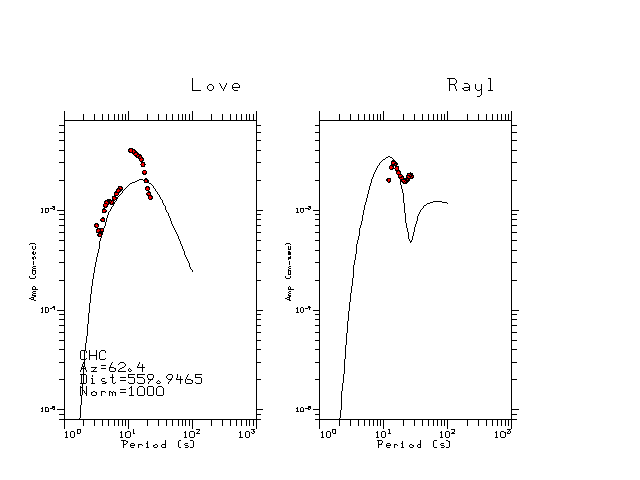
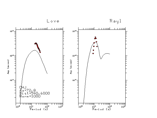
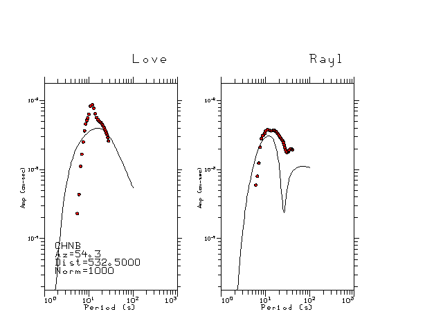
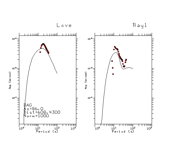
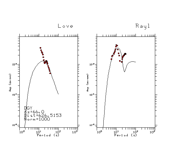
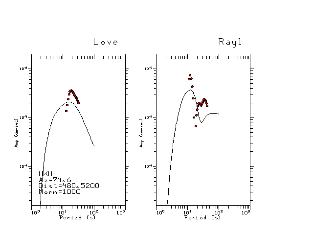
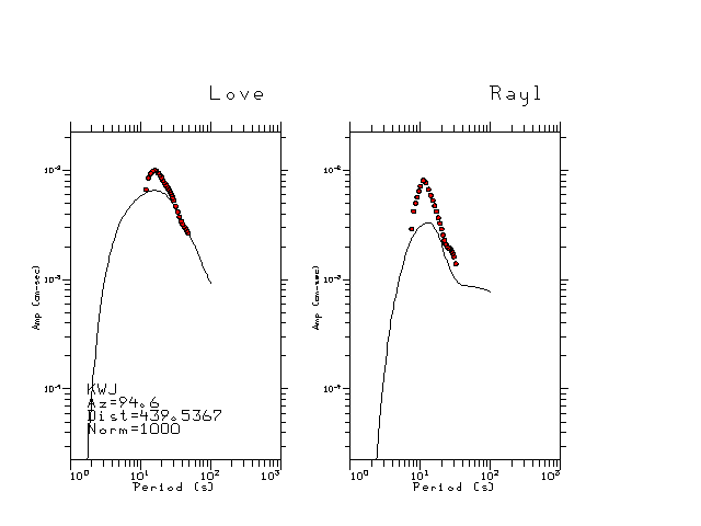
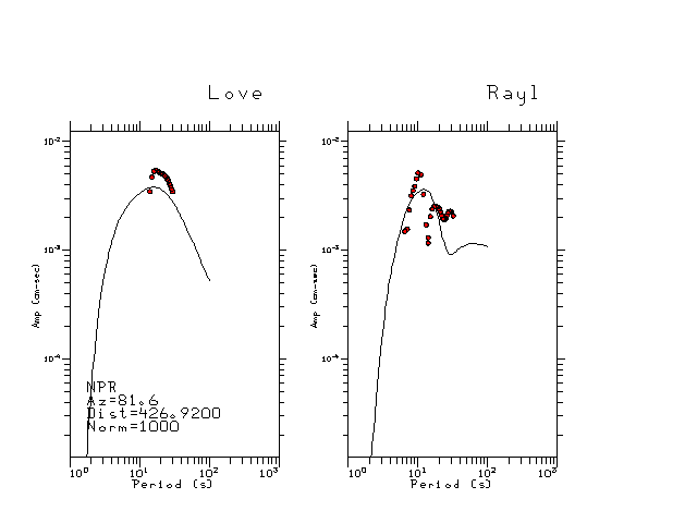
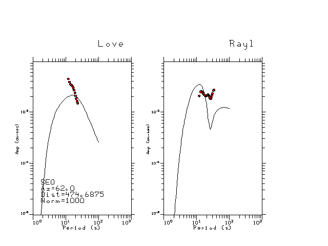
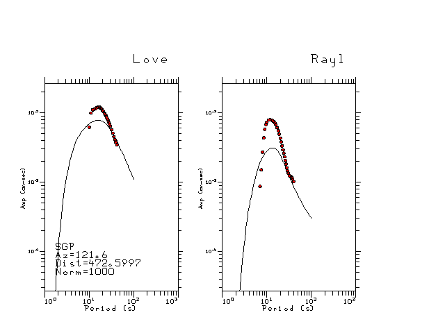
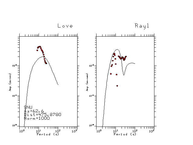
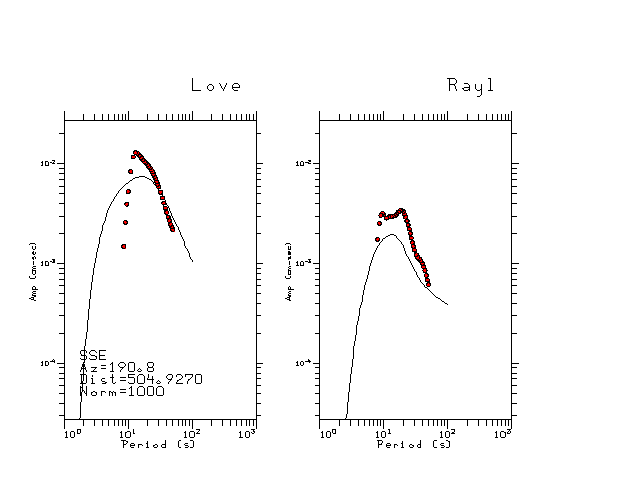
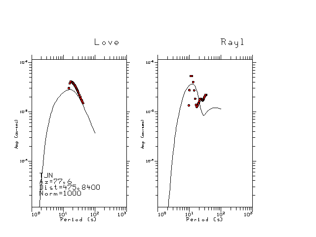
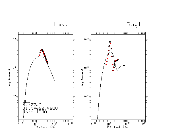
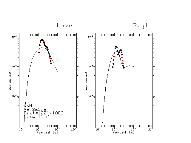
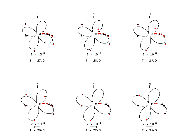
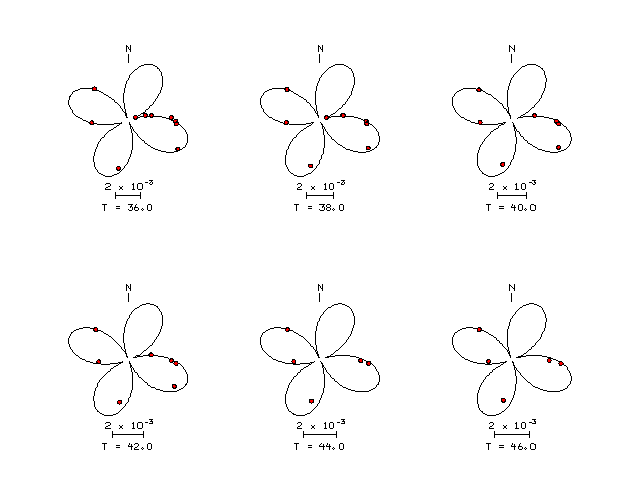
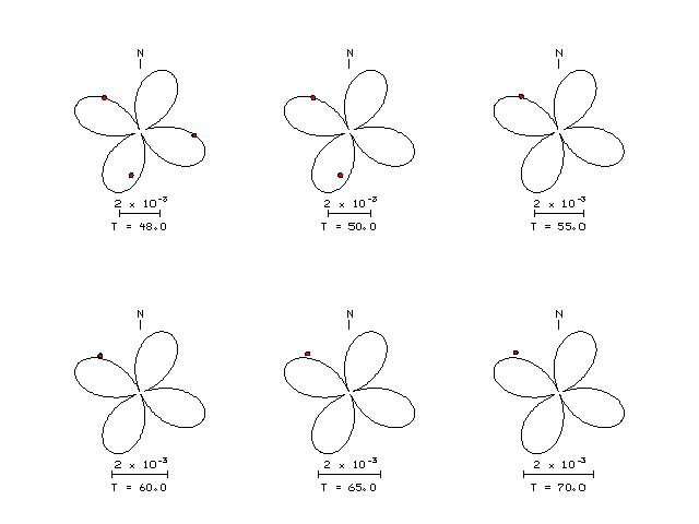
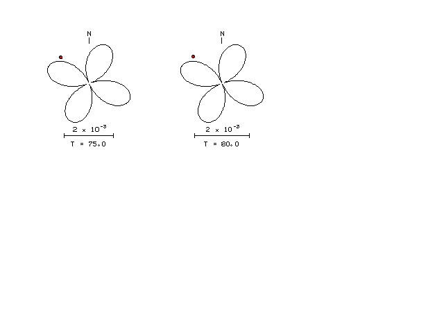
The figures below show the observed spectral amplitudes (units of cm-sec) at each station and the
theoretical predictions as a function of period for the mechanism given above. The modified Utah model earth model
was used to define the Green's functions. For each station, the Love and Rayleigh wave spectrail amplitudes are plotted with the same scaling so that one can get a sense fo the effects of the effects of the focal mechanism and depth on the excitation of each.
 |
 |
 |
 |
 |
 |
 |
 |
 |
 |
 |
 |
 |
 |
 |
 |
 |
 |
Here we tabulate the reasons for not using certain digital data sets