1999/04/07 14:43:18 37.20N 128.83E 2 3.70 Korea
 SLU Moment Tensor Solution
 1999/04/07 14:43:18 37.20N 128.83E 2 3.70 Korea

 Best Fitting Double Couple
    Mo = 3.98e+21 dyne-cm
    Mw = 3.70
    Z  = 2 km
     Plane   Strike  Dip  Rake
      NP1      203    80   -165
      NP2      110    75   -10
 Principal Axes:
   Axis    Value   Plunge  Azimuth
     T   3.98e+21      4     336
     N   0.00e+00     72     234
     P  -3.98e+21     18      67


 Moment Tensor: (dyne-cm)
    Component  Value
       Mxx     2.74e+21
       Mxy    -2.79e+21
       Mxz    -2.16e+20
       Myy    -2.39e+21
       Myz    -1.16e+21
       Mzz    -3.46e+20


                     ##############
                 # T ##############----
              ####   ############---------
             ###################-----------
           ####################--------------
          ####################----------------
         ####################-------------   --
        -###################-------------- P ---
        ---################---------------   ---
       -------############-----------------------
       ----------#########-----------------------
       -------------#####------------------------
       -----------------#------------------------
        ----------------######------------------
        ---------------##############-----------
         -------------#########################
          ------------########################
           ----------########################
             --------######################
              ------######################
                 ---###################
                     ##############


 Harvard Convention
 Moment Tensor:
      R          T          F
 -3.46e+20  -2.16e+20   1.16e+21
 -2.16e+20   2.74e+21   2.79e+21
  1.16e+21   2.79e+21  -2.39e+21
|
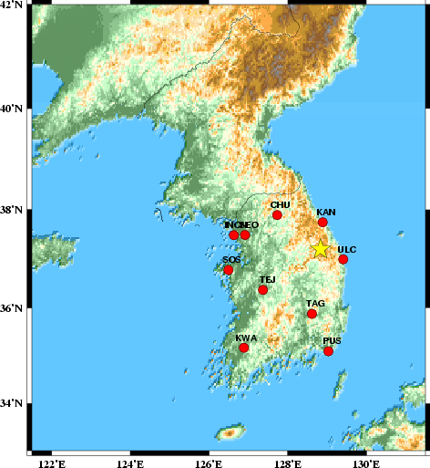
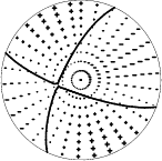
The focal mechanism was determined using broadband seismic waveforms. The location of the event and the station distribution are given in Figure 1.
|
|
|
|
      STK = 110
      DIP = 75
     RAKE = -10
       MW = 3.70
       HS = 2
The waveform inversion is preferred. This solution agrees with the surface-wave solution. This solution is well determined. Note that this date was duing the installation of the KMA network. Using the IRIS INCN station as a reference, it was determined that all KMA polarities should be flipped.
The program wvfgrd96 was used with good traces observed at short distance to determine the focal mechanism, depth and seismic moment. This technique requires a high quality signal and well determined velocity model for the Green functions. To the extent that these are the quality data, this type of mechanism should be preferred over the radiation pattern technique which requires the separate step of defining the pressure and tension quadrants and the correct strike.
The observed and predicted traces are filtered using the following gsac commands:
hp c 0.02 3
lp c 0.10 3
The results of this grid search from 0.5 to 19 km depth are as follow:
           DEPTH  STK   DIP  RAKE   MW    FIT
WVFGRD96    0.5   105    75   -15   3.67 0.6956
WVFGRD96    1.0   105    70   -15   3.69 0.7069
WVFGRD96    2.0   110    75   -10   3.70 0.7121
WVFGRD96    3.0   105    75   -15   3.72 0.7045
WVFGRD96    4.0   110    80   -15   3.73 0.6968
WVFGRD96    5.0   110    80   -15   3.74 0.6880
WVFGRD96    6.0   110    80    15   3.74 0.6784
WVFGRD96    7.0   110    85    15   3.75 0.6721
WVFGRD96    8.0   110    85    15   3.76 0.6665
WVFGRD96    9.0   110    85    15   3.76 0.6610
WVFGRD96   10.0   110    85    15   3.77 0.6554
WVFGRD96   11.0   110    85    15   3.78 0.6492
WVFGRD96   12.0   110    85    15   3.79 0.6418
WVFGRD96   13.0   110    85    15   3.79 0.6339
WVFGRD96   14.0   110    85    15   3.80 0.6261
WVFGRD96   15.0   285    80   -20   3.80 0.6178
WVFGRD96   16.0   285    80   -20   3.81 0.6129
WVFGRD96   17.0   285    80   -20   3.82 0.6082
WVFGRD96   18.0   285    80   -20   3.82 0.6038
WVFGRD96   19.0   285    80   -20   3.83 0.6010
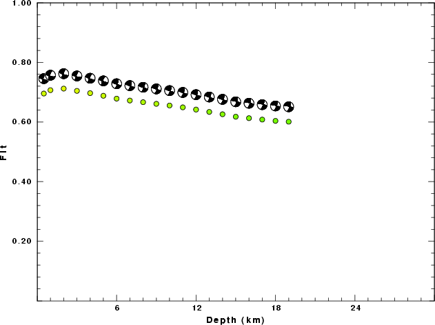
The best solution is
WVFGRD96 2.0 110 75 -10 3.70 0.7121
The mechanism correspond to the best fit is
|
|
|
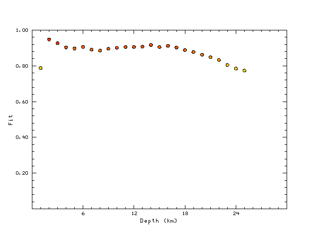
The best fit as a function of depth is given in the following figure:
|
|
|
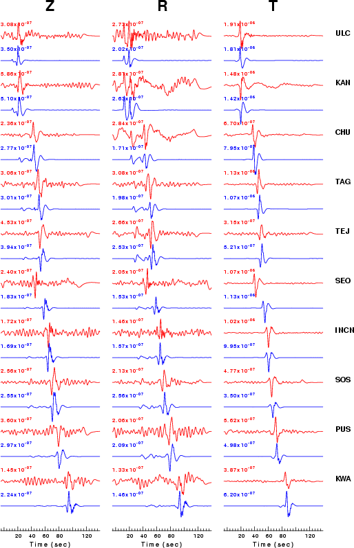
The comparison of the observed and predicted waveforms is given in the next figure. The red traces are the observed and the blue are the predicted. Each observed-predicted componnet is plotted to the same scale and peak amplitudes are indicated by the numbers to the left of each trace. The number in black at the rightr of each predicted traces it the time shift required for maximum correlation between the observed and predicted traces. This time shift is required because the synthetics are not computed at exactly the same distance as the observed and because the velocity model used in the predictions may not be perfect. A positive time shift indicates that the prediction is too fast and should be delayed to match the observed trace (shift to the right in this figure). A negative value indicates that the prediction is too slow. The bandpass filter used in the processing and for the display was
hp c 0.02 3
lp c 0.10 3

|
|
|
|
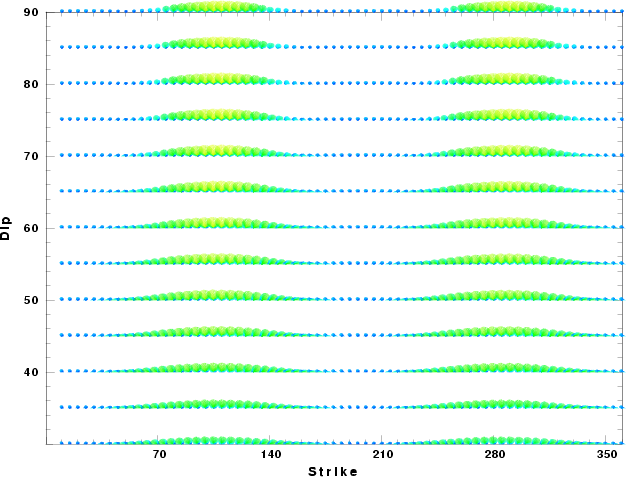
| Focal mechanism sensitivity at the preferred depth. The red color indicates a very good fit to thewavefroms. Each solution is plotted as a vector at a given value of strike and dip with the angle of the vector representing the rake angle, measured, with respect to the upward vertical (N) in the figure. |
  NODAL PLANES


  STK=     109.75
  DIP=      75.92
 RAKE=     159.36

             OR

  STK=     204.99
  DIP=      70.00
 RAKE=      15.00


DEPTH = 2.0 km

Mw = 3.70
Best Fit 0.9471 - P-T axis plot gives solutions with FIT greater than FIT90
 |
The P-wave first motion data for focal mechanism studies are as follow:
Sta Az(deg)    Dist(km)   First motion
ULC       114   57 iP_C
KAN         5   60 iP_C
CHU       309  124 eP_-
TAG       187  148 iP_C
TEJ       235  160 iP_D
SEO       281  173 iP_C
INCN      280  197 eP_-
SOS       258  213 eP_-
PUS       175  234 eP_X
KWA       218  285 eP_X
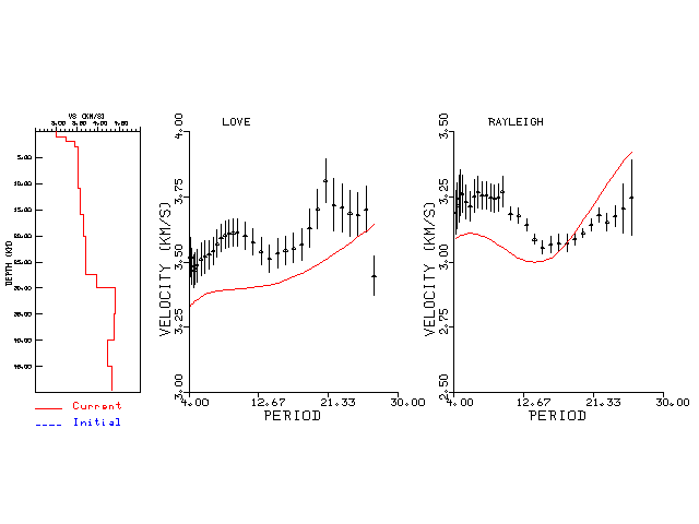
Surface wave analysis was performed using codes from Computer Programs in Seismology, specifically the multiple filter analysis program do_mft and the surface-wave radiation pattern search program srfgrd96.
Digital data were collected, instrument response removed and traces converted
to Z, R an T components. Multiple filter analysis was applied to the Z and T traces to obtain the Rayleigh- and Love-wave spectral amplitudes, respectively.
These were input to the search program which examined all depths between 1 and 25 km
and all possible mechanisms.
|
|
|
|
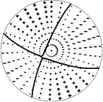
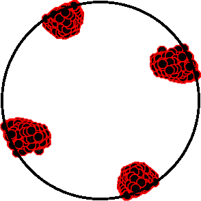
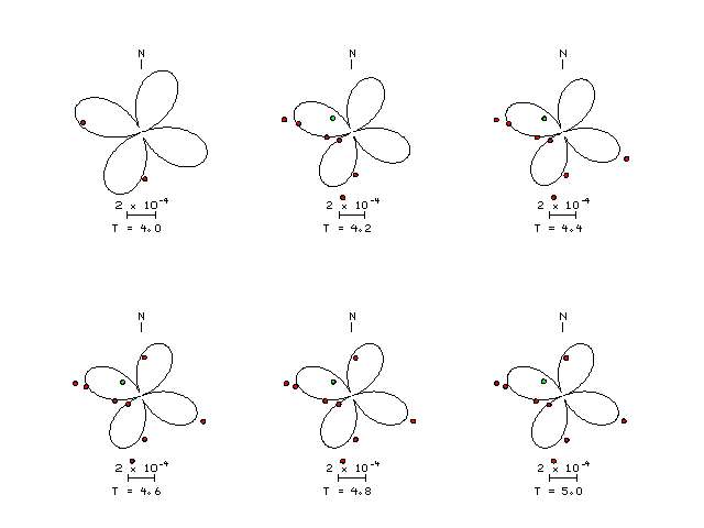
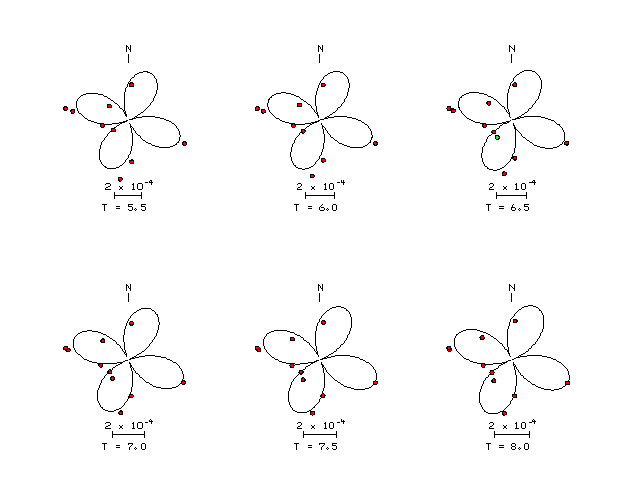
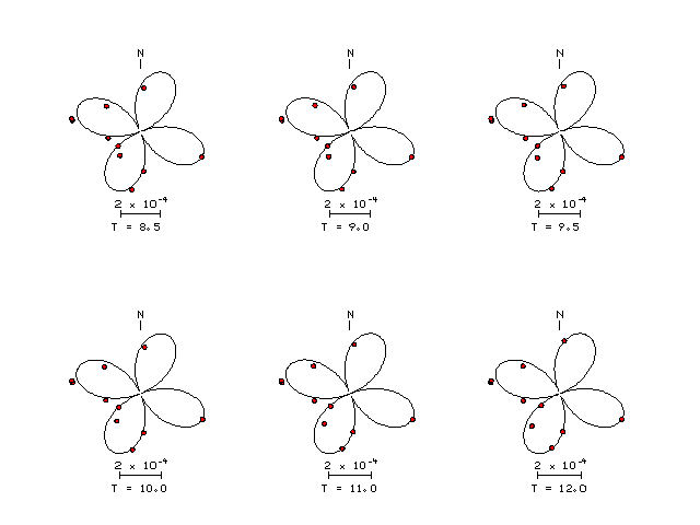
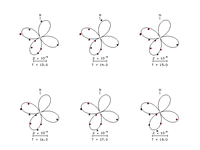
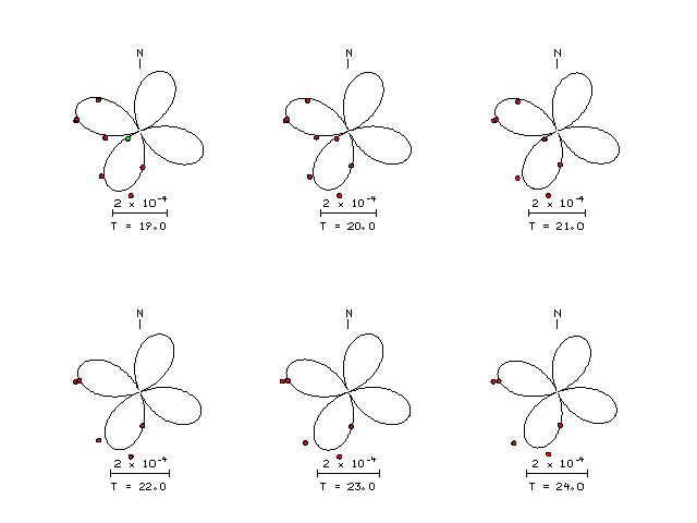
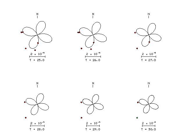
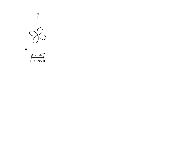
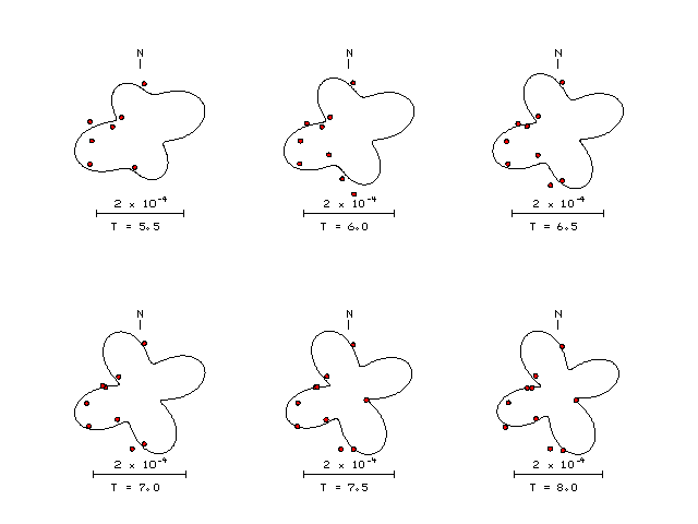
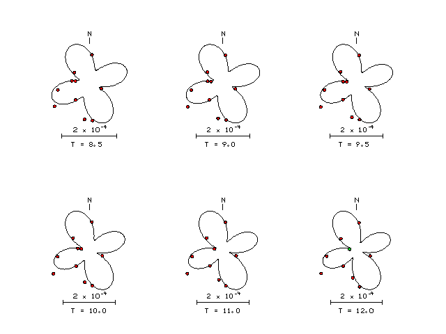
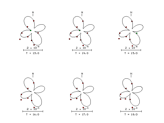
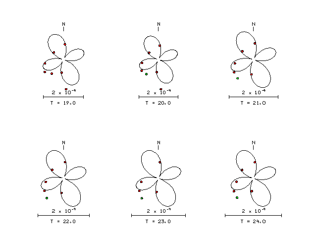
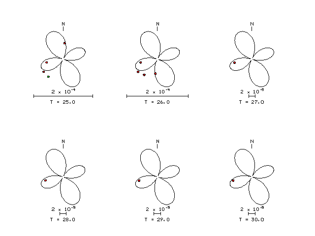
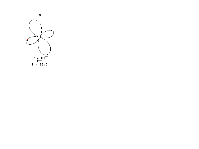
| Pressure-tension axis trends. Since the surface-wave spectra search does not distinguish between P and T axes and since there is a 180 ambiguity in strike, all possible P and T axes are plotted. First motion data and waveforms will be used to select the preferred mechanism. The purpose of this plot is to provide an idea of the possible range of solutions. The P and T-axes for all mechanisms with goodness of fit greater than 0.9 FITMAX (above) are plotted here. |
|
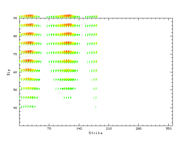
| Focal mechanism sensitivity at the preferred depth. The red color indicates a very good fit to the Love and Rayleigh wave radiation patterns. Each solution is plotted as a vector at a given value of strike and dip with the angle of the vector representing the rake angle, measured, with respect to the upward vertical (N) in the figure. Because of the symmetry of the spectral amplitude rediation patterns, only strikes from 0-180 degrees are sampled. |
The distribution of broadband stations with azimuth and distance is
Sta Az(deg)    Dist(km)
ULC	  114	   57
KAN	    5	   60
CHU	  309	  124
TAG	  187	  148
TEJ	  235	  160
SEO	  281	  173
INCN	  280	  197
SOS	  258	  213
PUS	  176	  234
KWA	  218	  285
Since the analysis of the surface-wave radiation patterns uses only spectral amplitudes and because the surfave-wave radiation patterns have a 180 degree symmetry, each surface-wave solution consists of four possible focal mechanisms corresponding to the interchange of the P- and T-axes and a roation of the mechanism by 180 degrees. To select one mechanism, P-wave first motion can be used. This was not possible in this case because all the P-wave first motions were emergent ( a feature of the P-wave wave takeoff angle, the station location and the mechanism). The other way to select among the mechanisms is to compute forward synthetics and compare the observed and predicted waveforms.
The fits to the waveforms with the given mechanism are show below:
|
This figure shows the fit to the three components of motion (Z - vertical, R-radial and T - transverse). For each station and component, the observed traces is shown in red and the model predicted trace in blue. The traces represent filtered ground velocity in units of meters/sec (the peak value is printed adjacent to each trace; each pair of traces to plotted to the same scale to emphasize the difference in levels). Both synthetic and observed traces have been filtered using the SAC commands:
hp c 0.02 3
lp c 0.10 3
|
|
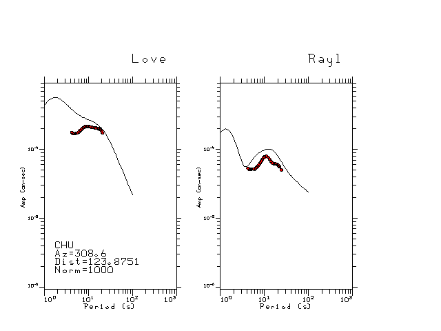
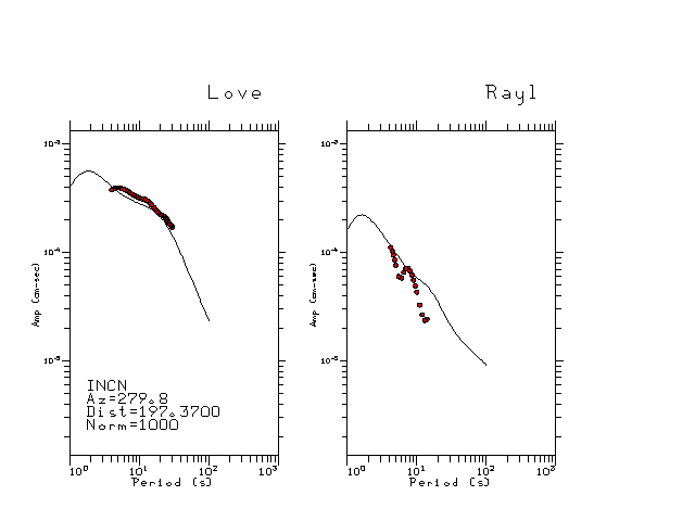
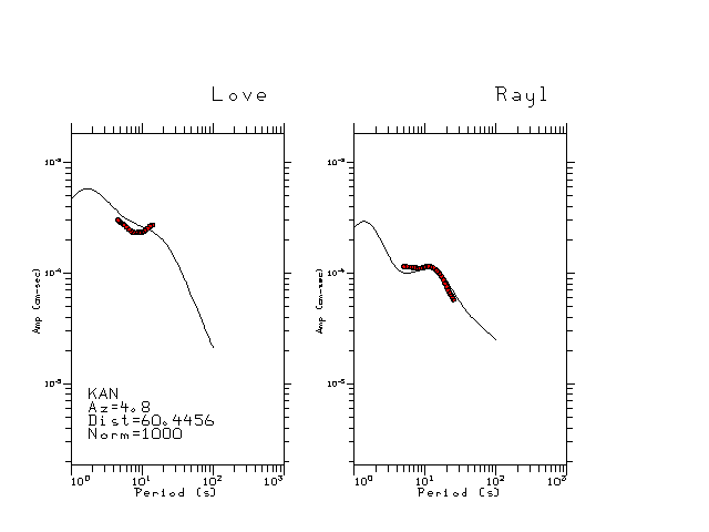
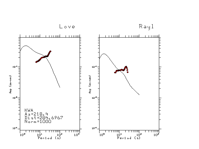
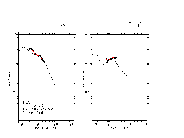
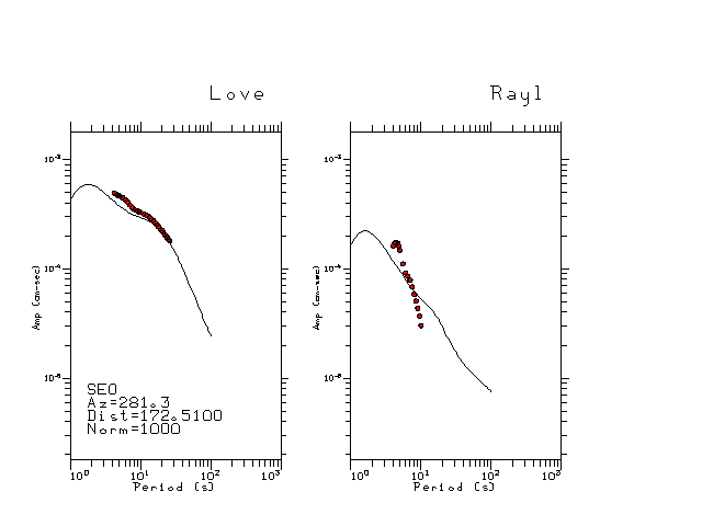
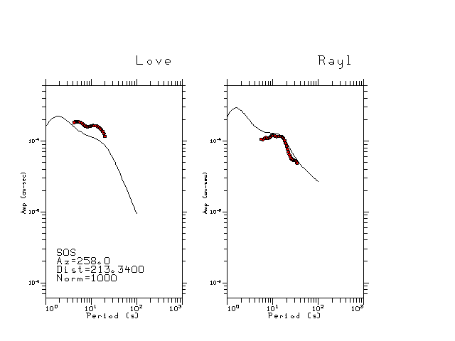
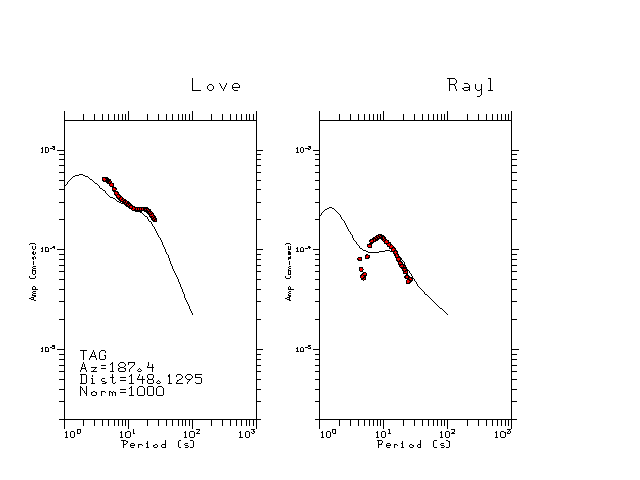
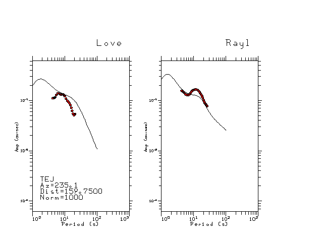
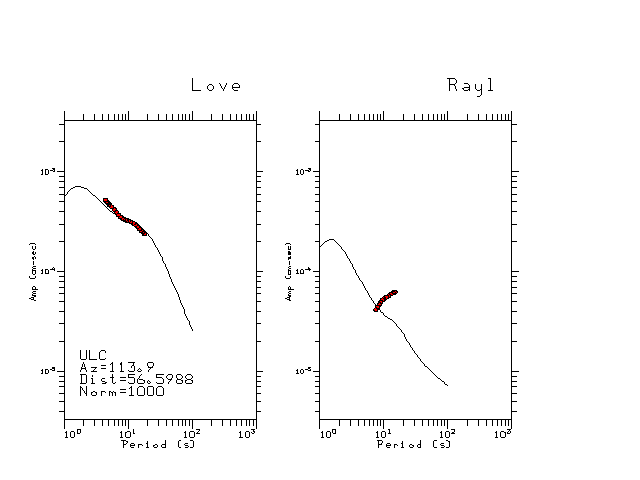
The figures below show the observed spectral amplitudes (units of cm-sec) at each station and the
theoretical predictions as a function of period for the mechanism given above. The modified Utah model earth model
was used to define the Green's functions. For each station, the Love and Rayleigh wave spectrail amplitudes are plotted with the same scaling so that one can get a sense fo the effects of the effects of the focal mechanism and depth on the excitation of each.
 |
 |
 |
 |
 |
 |
 |
 |
 |
 |
Here we tabulate the reasons for not using certain digital data sets