Location

2019/11/07 17:35:21 41.78 13.61 14.0 4.4 Balsorano (AQ)

Arrival Times (from USGS)

Felt Map

Focal Mechanism

SLU Moment Tensor Solution ENS 2019/11/07 17:35:21:0 41.78 13.61 14.0 4.4 Balsorano (AQ) Stations used: IV.ARCI IV.ARVD IV.ATFO IV.ATMI IV.ATTE IV.CAMP IV.CERA IV.CERT IV.CESI IV.CESX IV.CRE IV.FAGN IV.FDMO IV.FIAM IV.GIUL IV.INTR IV.LATE IV.LAV9 IV.LPEL IV.MA9 IV.MGAB IV.MIDA IV.MOMA IV.MTCE IV.OFFI IV.PARC IV.PESA IV.PIEI IV.PIGN IV.PTQR IV.PTRJ IV.RMP IV.RNI2 IV.SACR IV.SACS IV.SNTG IV.SSFR IV.TERO IV.TRTR IV.VAGA MN.AQU Filtering commands used: cut o DIST/3.3 -20 o DIST/3.3 +50 rtr taper w 0.1 hp c 0.03 n 3 lp c 0.10 n 3 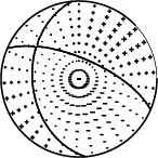Best Fitting Double Couple Mo = 7.08e+22 dyne-cm Mw = 4.50 Z = 15 km Plane Strike Dip Rake NP1 293 68 -125 NP2 175 40 -35 Principal Axes: Axis Value Plunge Azimuth T 7.08e+22 16 48 N 0.00e+00 32 307 P -7.08e+22 53 161 Moment Tensor: (dyne-cm) Component Value Mxx 6.78e+21 Mxy 4.02e+22 Mxz 4.49e+22 Myy 3.32e+22 Myz 3.15e+21 Mzz -4.00e+22 ---########### -----################# ------###################### ------##################### -------###################### T ## -------####################### ### ########--############################ ########-----------##################### ########---------------################# #########-------------------############## #########----------------------########### #########-------------------------######## #########---------------------------###### ########-----------------------------### #########------------ --------------## ########------------ P --------------- ########----------- -------------- ########-------------------------- #######----------------------- ########-------------------- #######--------------- ######-------- Global CMT Convention Moment Tensor: R T P -4.00e+22 4.49e+22 -3.15e+21 4.49e+22 6.78e+21 -4.02e+22 -3.15e+21 -4.02e+22 3.32e+22 Details of the solution is found at http://www.eas.slu.edu/eqc/eqc_mt/MECH.IT/20191107173521/index.html

Preferred Solution

The preferred solution from an analysis of the surface-wave spectral amplitude radiation pattern, waveform inversion and first motion observations is

      STK = 175
      DIP = 40
     RAKE = -35
       MW = 4.50
       HS = 15.0

The NDK file is 20191107173521.ndk The waveform inversion is preferred.

Moment Tensor Comparison

The following compares this source inversion to others

SLU INGVTDMT

SLU Moment Tensor Solution ENS 2019/11/07 17:35:21:0 41.78 13.61 14.0 4.4 Balsorano (AQ) Stations used: IV.ARCI IV.ARVD IV.ATFO IV.ATMI IV.ATTE IV.CAMP IV.CERA IV.CERT IV.CESI IV.CESX IV.CRE IV.FAGN IV.FDMO IV.FIAM IV.GIUL IV.INTR IV.LATE IV.LAV9 IV.LPEL IV.MA9 IV.MGAB IV.MIDA IV.MOMA IV.MTCE IV.OFFI IV.PARC IV.PESA IV.PIEI IV.PIGN IV.PTQR IV.PTRJ IV.RMP IV.RNI2 IV.SACR IV.SACS IV.SNTG IV.SSFR IV.TERO IV.TRTR IV.VAGA MN.AQU Filtering commands used: cut o DIST/3.3 -20 o DIST/3.3 +50 rtr taper w 0.1 hp c 0.03 n 3 lp c 0.10 n 3 Best Fitting Double Couple Mo = 7.08e+22 dyne-cm Mw = 4.50 Z = 15 km Plane Strike Dip Rake NP1 293 68 -125 NP2 175 40 -35 Principal Axes: Axis Value Plunge Azimuth T 7.08e+22 16 48 N 0.00e+00 32 307 P -7.08e+22 53 161 Moment Tensor: (dyne-cm) Component Value Mxx 6.78e+21 Mxy 4.02e+22 Mxz 4.49e+22 Myy 3.32e+22 Myz 3.15e+21 Mzz -4.00e+22 ---########### -----################# ------###################### ------##################### -------###################### T ## -------####################### ### ########--############################ ########-----------##################### ########---------------################# #########-------------------############## #########----------------------########### #########-------------------------######## #########---------------------------###### ########-----------------------------### #########------------ --------------## ########------------ P --------------- ########----------- -------------- ########-------------------------- #######----------------------- ########-------------------- #######--------------- ######-------- Global CMT Convention Moment Tensor: R T P -4.00e+22 4.49e+22 -3.15e+21 4.49e+22 6.78e+21 -4.02e+22 -3.15e+21 -4.02e+22 3.32e+22 Details of the solution is found at http://www.eas.slu.edu/eqc/eqc_mt/MECH.IT/20191107173521/index.html

Magnitudes

ML Magnitude

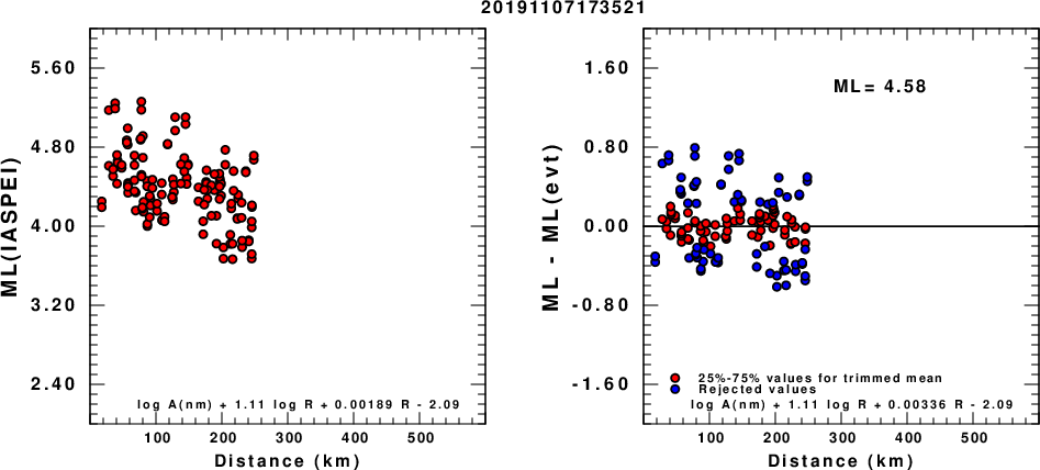
(a) ML computed using the IASPEI formula for Horizontal components; (b) ML residuals computed using a modified IASPEI formula that accounts for path specific attenuation; the values used for the trimmed mean are indicated. The ML relation used for each figure is given at the bottom of each plot.

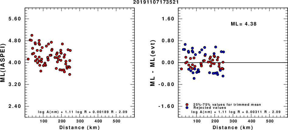
(a) ML computed using the IASPEI formula for Vertical components (research); (b) ML residuals computed using a modified IASPEI formula that accounts for path specific attenuation; the values used for the trimmed mean are indicated. The ML relation used for each figure is given at the bottom of each plot.

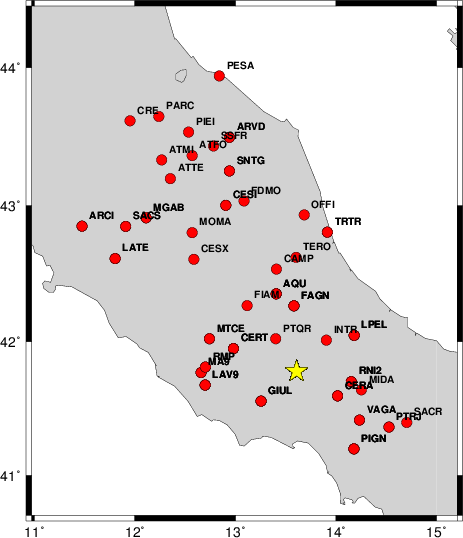
Waveform Inversion

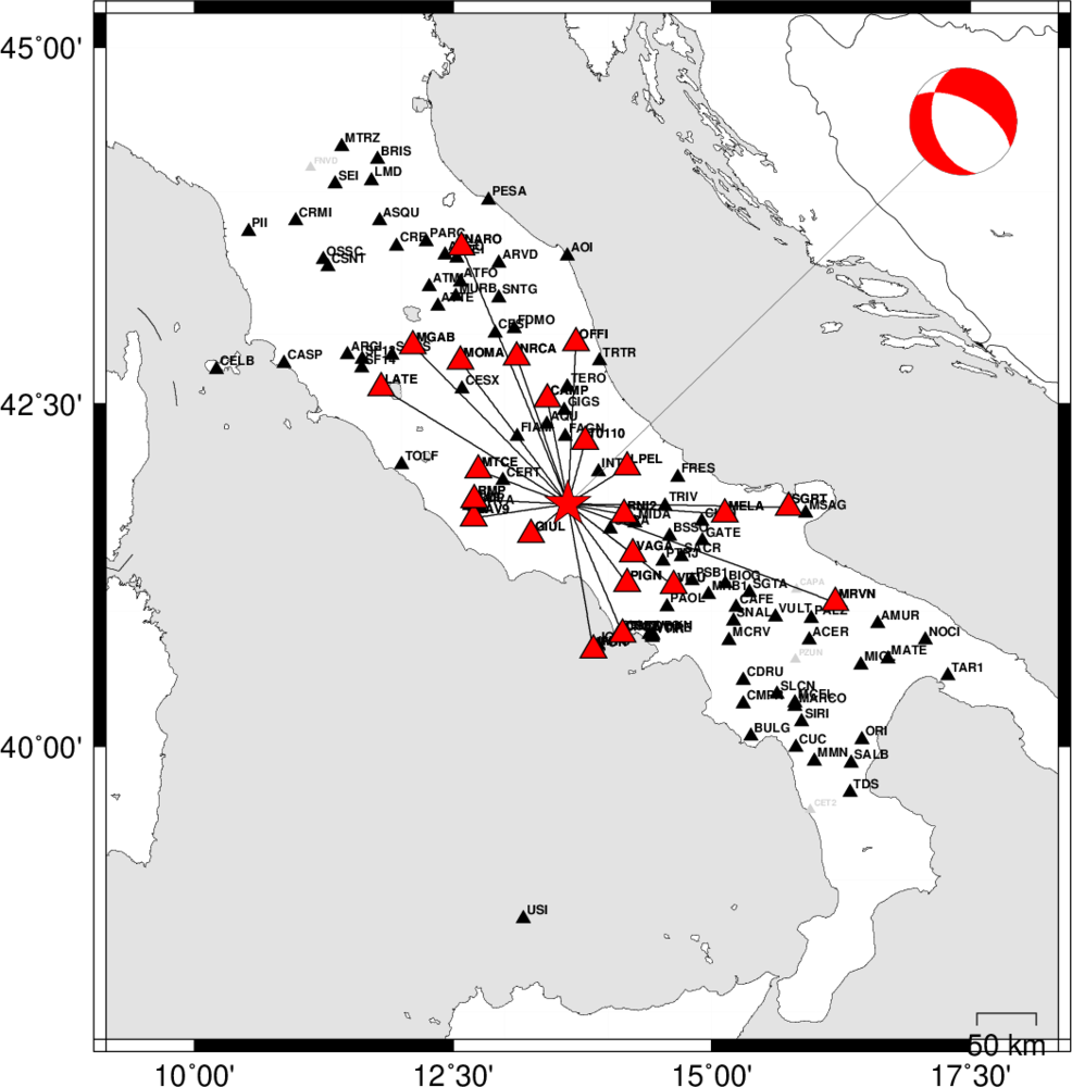
The focal mechanism was determined using broadband seismic waveforms. The location of the event and the and stations used for the waveform inversion are shown in the next figure.

Location of broadband stations used for waveform inversion

The program wvfgrd96 was used with good traces observed at short distance to determine the focal mechanism, depth and seismic moment. This technique requires a high quality signal and well determined velocity model for the Green functions. To the extent that these are the quality data, this type of mechanism should be preferred over the radiation pattern technique which requires the separate step of defining the pressure and tension quadrants and the correct strike.

The observed and predicted traces are filtered using the following gsac commands:

cut o DIST/3.3 -20 o DIST/3.3 +50
rtr
taper w 0.1
hp c 0.03 n 3 
lp c 0.10 n 3

The results of this grid search from 0.5 to 19 km depth are as follow:

           DEPTH  STK   DIP  RAKE   MW    FIT
WVFGRD96    1.0    55    45    90   4.14 0.3034
WVFGRD96    2.0   200    60    45   4.18 0.3242
WVFGRD96    3.0     0    55   -20   4.21 0.3501
WVFGRD96    4.0     0    60   -20   4.24 0.3856
WVFGRD96    5.0   355    50   -30   4.33 0.4199
WVFGRD96    6.0   180    40   -25   4.37 0.4541
WVFGRD96    7.0   175    35   -35   4.40 0.4958
WVFGRD96    8.0   180    45   -30   4.38 0.5194
WVFGRD96    9.0   180    45   -30   4.39 0.5391
WVFGRD96   10.0   180    45   -30   4.41 0.5535
WVFGRD96   11.0   180    45   -30   4.42 0.5629
WVFGRD96   12.0   180    45   -30   4.43 0.5681
WVFGRD96   13.0   180    45   -30   4.45 0.5696
WVFGRD96   14.0   180    45   -30   4.46 0.5677
WVFGRD96   15.0   175    40   -35   4.50 0.5726
WVFGRD96   16.0   175    40   -35   4.51 0.5669
WVFGRD96   17.0   175    45   -35   4.51 0.5594
WVFGRD96   18.0   175    45   -35   4.52 0.5498
WVFGRD96   19.0   175    45   -35   4.53 0.5385

The best solution is

WVFGRD96   15.0   175    40   -35   4.50 0.5726

The mechanism correspond to the best fit is

Figure 1. Waveform inversion focal mechanism

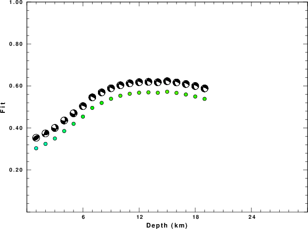
The best fit as a function of depth is given in the following figure:

Figure 2. Depth sensitivity for waveform mechanism

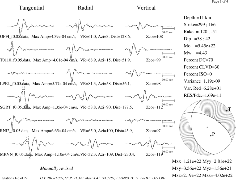
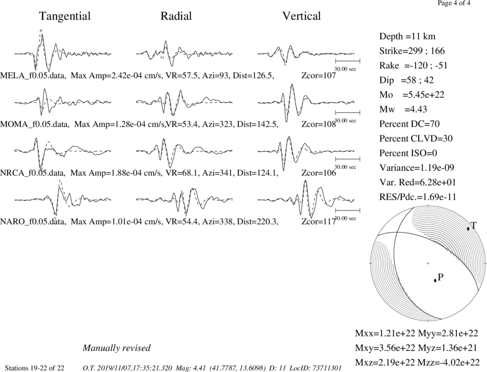
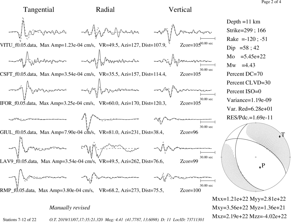
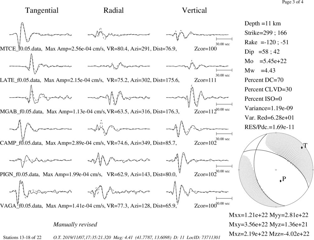
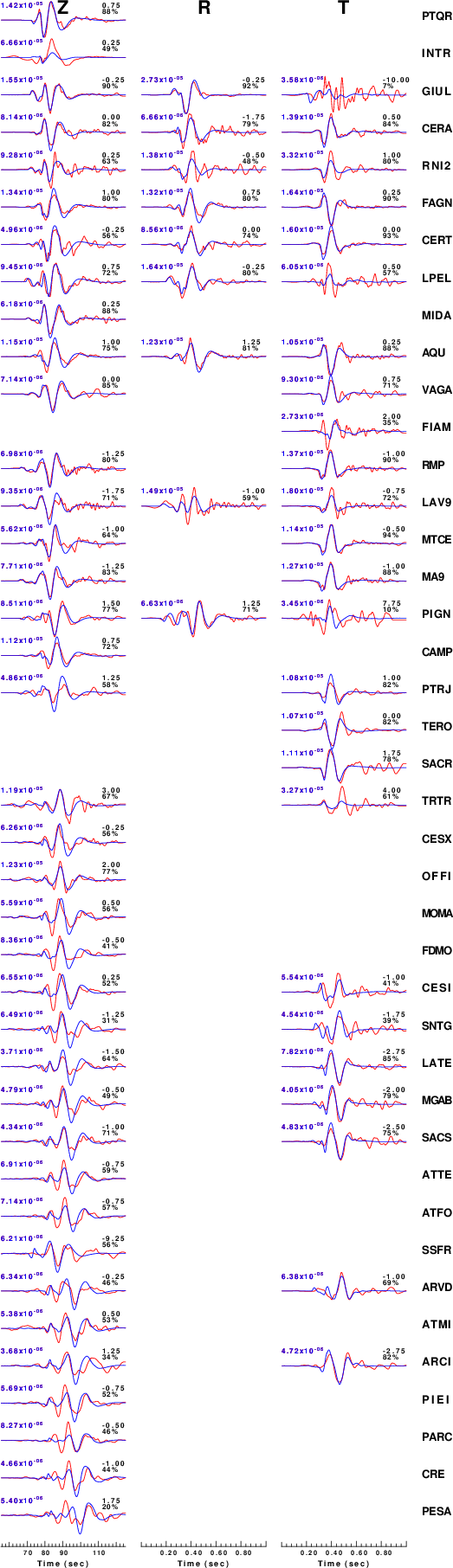
The comparison of the observed and predicted waveforms is given in the next figure. The red traces are the observed and the blue are the predicted. Each observed-predicted component is plotted to the same scale and peak amplitudes are indicated by the numbers to the left of each trace. A pair of numbers is given in black at the right of each predicted traces. The upper number it the time shift required for maximum correlation between the observed and predicted traces. This time shift is required because the synthetics are not computed at exactly the same distance as the observed and because the velocity model used in the predictions may not be perfect. A positive time shift indicates that the prediction is too fast and should be delayed to match the observed trace (shift to the right in this figure). A negative value indicates that the prediction is too slow. The lower number gives the percentage of variance reduction to characterize the individual goodness of fit (100% indicates a perfect fit).

The bandpass filter used in the processing and for the display was

cut o DIST/3.3 -20 o DIST/3.3 +50
rtr
taper w 0.1
hp c 0.03 n 3 
lp c 0.10 n 3

Figure 3. Waveform comparison for selected depth. Red: observed; Blue - predicted. The time shift with respect to the model prediction is indicated. The percent of fit is also indicated.

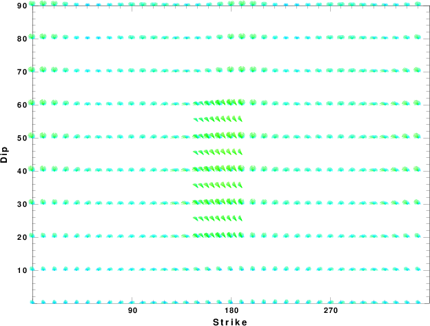
Focal mechanism sensitivity at the preferred depth. The red color indicates a very good fit to thewavefroms. Each solution is plotted as a vector at a given value of strike and dip with the angle of the vector representing the rake angle, measured, with respect to the upward vertical (N) in the figure.

A check on the assumed source location is possible by looking at the time shifts between the observed and predicted traces. The time shifts for waveform matching arise for several reasons:

The origin time and epicentral distance are incorrect
The velocity model used for the inversion is incorrect
The velocity model used to define the P-arrival time is not the same as the velocity model used for the waveform inversion (assuming that the initial trace alignment is based on the P arrival time)

Assuming only a mislocation, the time shifts are fit to a functional form:

 Time_shift = A + B cos Azimuth + C Sin Azimuth

The time shifts for this inversion lead to the next figure:

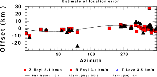
The derived shift in origin time and epicentral coordinates are given at the bottom of the figure.

Discussion

Velocity Model

The nnCIA used for the waveform synthetic seismograms and for the surface wave eigenfunctions and dispersion is as follows:

MODEL.01
C.It. A. Di Luzio et al Earth Plan Lettrs 280 (2009) 1-12 Fig 5. 7-8 MODEL/SURF3
ISOTROPIC
KGS
FLAT EARTH
1-D
CONSTANT VELOCITY
LINE08
LINE09
LINE10
LINE11
      H(KM)   VP(KM/S)   VS(KM/S) RHO(GM/CC)         QP         QS       ETAP       ETAS      FREFP      FREFS
     1.5000     3.7497     2.1436     2.2753  0.500E-02  0.100E-01   0.00       0.00       1.00       1.00    
     3.0000     4.9399     2.8210     2.4858  0.500E-02  0.100E-01   0.00       0.00       1.00       1.00    
     3.0000     6.0129     3.4336     2.7058  0.500E-02  0.100E-01   0.00       0.00       1.00       1.00    
     7.0000     5.5516     3.1475     2.6093  0.167E-02  0.333E-02   0.00       0.00       1.00       1.00    
    15.0000     5.8805     3.3583     2.6770  0.167E-02  0.333E-02   0.00       0.00       1.00       1.00    
     6.0000     7.1059     4.0081     3.0002  0.167E-02  0.333E-02   0.00       0.00       1.00       1.00    
     8.0000     7.1000     3.9864     3.0120  0.167E-02  0.333E-02   0.00       0.00       1.00       1.00    
     0.0000     7.9000     4.4036     3.2760  0.167E-02  0.333E-02   0.00       0.00       1.00       1.00

Quality Control

Here we tabulate the reasons for not using certain digital data sets

The following stations did not have a valid response files:

DATE=Thu Nov 7 20:43:48 CST 2019

Last Changed 2019/11/07