Location
2019/01/14 23:03:56 44.37 12.32 25.0 4.3 Ravena (RA)
Arrival Times (from USGS)
Arrival time list
Felt Map
USGS Felt map for this earthquake
USGS Felt reports page for
Focal Mechanism
 SLU Moment Tensor Solution
 ENS  2019/01/14 23:03:56:0  44.37   12.32  25.0 4.3 Ravena (RA)

 Stations used:
   CH.BERNI CH.FUORN CH.PANIX CH.PLONS CH.VDL GU.POPM IV.APEC
   IV.ARVD IV.ASSB IV.ATFO IV.ATMI IV.ATPC IV.ATTE IV.ATVO
   IV.BDI IV.BRIS IV.CAFI IV.CELB IV.CESX IV.CRE IV.CSNT
   IV.CTI IV.FDMO IV.FIAM IV.FNVD IV.GUMA IV.LATE IV.LMD
   IV.MAGA IV.MGAB IV.MOMA IV.MTRZ IV.MURB IV.NARO IV.NRCA
   IV.OFFI IV.OSSC IV.PARC IV.PIEI IV.PII IV.PLMA IV.SNTG
   IV.SSFR IV.VIVA MN.TRI MN.TUE MN.VLC NI.PALA NI.VINO
   OX.BALD OX.DRE RD.PGF SI.BOSI SI.KOSI SI.LUSI SI.MOSI
   SI.ROSI ST.DOSS

 Filtering commands used:
   cut o DIST/3.3 -20 o DIST/3.3 +50
   rtr
   taper w 0.1
   hp c 0.02 n 3
   lp c 0.05 n 3

 Best Fitting Double Couple
  Mo = 4.84e+22 dyne-cm
  Mw = 4.39
  Z  = 16 km
  Plane   Strike  Dip  Rake
   NP1      312    56    97
   NP2      120    35    80
  Principal Axes:
   Axis    Value   Plunge  Azimuth
    T   4.84e+22     78     247
    N   0.00e+00      6     128
    P  -4.84e+22     10      37

 Moment Tensor: (dyne-cm)
    Component   Value
       Mxx    -2.94e+22
       Mxy    -2.18e+22
       Mxz    -1.07e+22
       Myy    -1.54e+22
       Myz    -1.41e+22
       Mzz     4.48e+22


                     --------------
                 --------------------
              ----------------------- P --
             #######-----------------   ---
           ##############--------------------
          ###################-----------------
         -######################---------------
        --########################--------------
        --##########################------------
       ---###########################------------
       ----#############   ############----------
       ----############# T #############---------
       -----############   ##############--------
        -----#############################------
        -------############################-----
         --------##########################----
          ---------########################---
           -----------#####################-#
             -------------##############---
              ----------------------------
                 ----------------------
                     --------------


 Global CMT Convention Moment Tensor:
      R          T          P
  4.48e+22  -1.07e+22   1.41e+22
 -1.07e+22  -2.94e+22   2.18e+22
  1.41e+22   2.18e+22  -1.54e+22


Details of the solution is found at

http://www.eas.slu.edu/eqc/eqc_mt/MECH.IT/20190114230356/index.html
|
Preferred Solution
The preferred solution from an analysis of the surface-wave spectral amplitude radiation pattern, waveform inversion and first motion observations is
      STK = 120
      DIP = 35
     RAKE = 80
       MW = 4.39
       HS = 16.0
The NDK file is 20190114230356.ndk
The RESP files wrom WebD3 for INGV (e.g., MAGA) were incorrect. The problem was that the Stage 3 FIR has a gain that was huge instead of 1.0. I used the pole-zero which ignores the FIR. evalresp could not be used
Moment Tensor Comparison
The following compares this source inversion to others
| SLU |
INGVTDMT |
 SLU Moment Tensor Solution
 ENS  2019/01/14 23:03:56:0  44.37   12.32  25.0 4.3 Ravena (RA)

 Stations used:
   CH.BERNI CH.FUORN CH.PANIX CH.PLONS CH.VDL GU.POPM IV.APEC
   IV.ARVD IV.ASSB IV.ATFO IV.ATMI IV.ATPC IV.ATTE IV.ATVO
   IV.BDI IV.BRIS IV.CAFI IV.CELB IV.CESX IV.CRE IV.CSNT
   IV.CTI IV.FDMO IV.FIAM IV.FNVD IV.GUMA IV.LATE IV.LMD
   IV.MAGA IV.MGAB IV.MOMA IV.MTRZ IV.MURB IV.NARO IV.NRCA
   IV.OFFI IV.OSSC IV.PARC IV.PIEI IV.PII IV.PLMA IV.SNTG
   IV.SSFR IV.VIVA MN.TRI MN.TUE MN.VLC NI.PALA NI.VINO
   OX.BALD OX.DRE RD.PGF SI.BOSI SI.KOSI SI.LUSI SI.MOSI
   SI.ROSI ST.DOSS

 Filtering commands used:
   cut o DIST/3.3 -20 o DIST/3.3 +50
   rtr
   taper w 0.1
   hp c 0.02 n 3
   lp c 0.05 n 3

 Best Fitting Double Couple
  Mo = 4.84e+22 dyne-cm
  Mw = 4.39
  Z  = 16 km
  Plane   Strike  Dip  Rake
   NP1      312    56    97
   NP2      120    35    80
  Principal Axes:
   Axis    Value   Plunge  Azimuth
    T   4.84e+22     78     247
    N   0.00e+00      6     128
    P  -4.84e+22     10      37

 Moment Tensor: (dyne-cm)
    Component   Value
       Mxx    -2.94e+22
       Mxy    -2.18e+22
       Mxz    -1.07e+22
       Myy    -1.54e+22
       Myz    -1.41e+22
       Mzz     4.48e+22


                     --------------
                 --------------------
              ----------------------- P --
             #######-----------------   ---
           ##############--------------------
          ###################-----------------
         -######################---------------
        --########################--------------
        --##########################------------
       ---###########################------------
       ----#############   ############----------
       ----############# T #############---------
       -----############   ##############--------
        -----#############################------
        -------############################-----
         --------##########################----
          ---------########################---
           -----------#####################-#
             -------------##############---
              ----------------------------
                 ----------------------
                     --------------


 Global CMT Convention Moment Tensor:
      R          T          P
  4.48e+22  -1.07e+22   1.41e+22
 -1.07e+22  -2.94e+22   2.18e+22
  1.41e+22   2.18e+22  -1.54e+22


Details of the solution is found at

http://www.eas.slu.edu/eqc/eqc_mt/MECH.IT/20190114230356/index.html
|
|
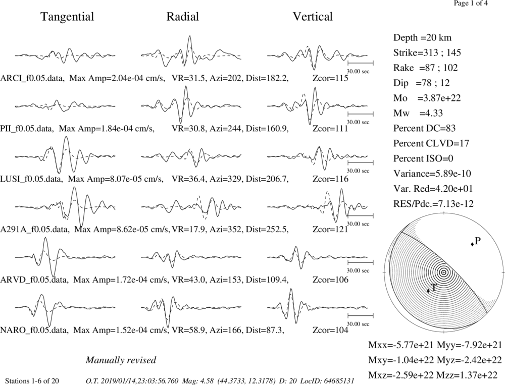
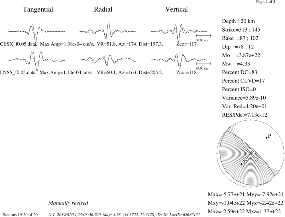
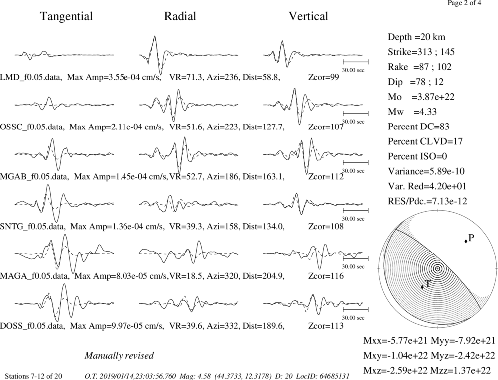
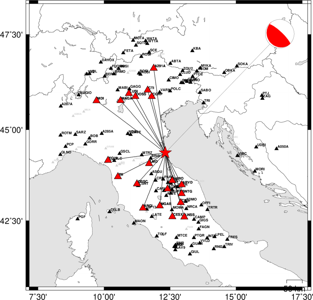
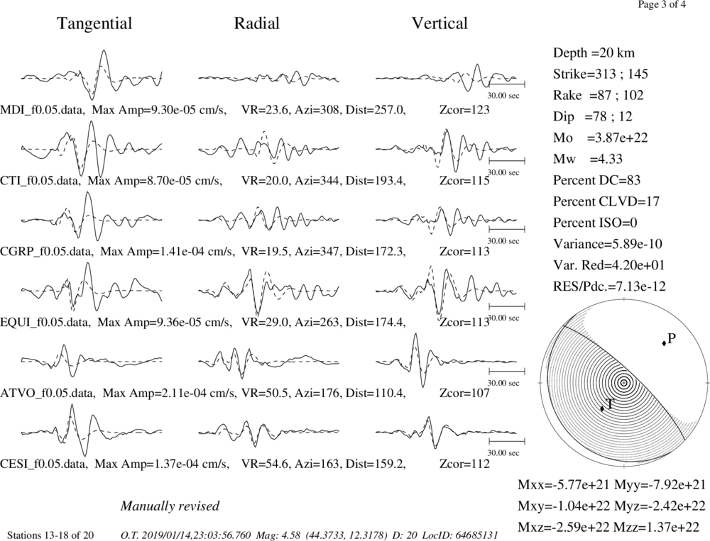
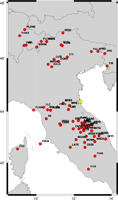
Waveform Inversion
The focal mechanism was determined using broadband seismic waveforms. The location of the event and the
and stations used for the waveform inversion are shown in the next figure.
|
|
Location of broadband stations used for waveform inversion
|
The program wvfgrd96 was used with good traces observed at short distance to determine the focal mechanism, depth and seismic moment. This technique requires a high quality signal and well determined velocity model for the Green functions. To the extent that these are the quality data, this type of mechanism should be preferred over the radiation pattern technique which requires the separate step of defining the pressure and tension quadrants and the correct strike.
The observed and predicted traces are filtered using the following gsac commands:
cut o DIST/3.3 -20 o DIST/3.3 +50
rtr
taper w 0.1
hp c 0.02 n 3
lp c 0.05 n 3
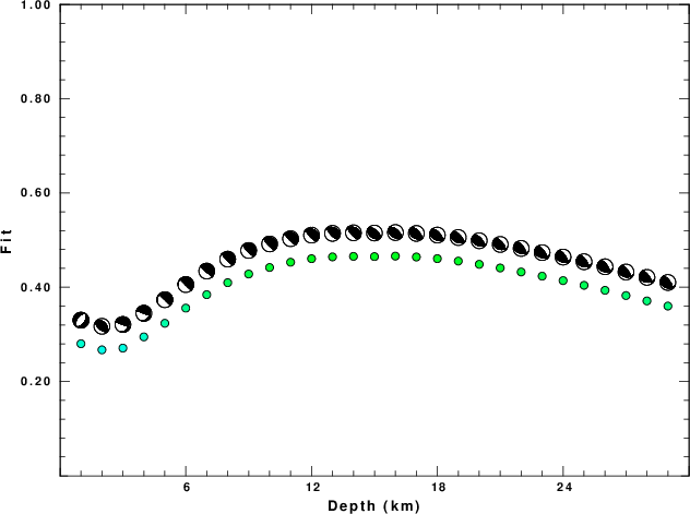
The results of this grid search from 0.5 to 19 km depth are as follow:
           DEPTH  STK   DIP  RAKE   MW    FIT
WVFGRD96    1.0    35    45   -90   4.18 0.2802
WVFGRD96    2.0   130    50    85   4.21 0.2672
WVFGRD96    3.0   110    90    65   4.32 0.2710
WVFGRD96    4.0   290    90   -65   4.30 0.2948
WVFGRD96    5.0   135    90    95   4.43 0.3236
WVFGRD96    6.0   250     5    25   4.41 0.3557
WVFGRD96    7.0   330    10   110   4.40 0.3843
WVFGRD96    8.0   300    15    75   4.35 0.4097
WVFGRD96    9.0   295    15    70   4.35 0.4281
WVFGRD96   10.0   300    20    75   4.36 0.4419
WVFGRD96   11.0   295    20    70   4.36 0.4531
WVFGRD96   12.0   295    25    70   4.36 0.4606
WVFGRD96   13.0   295    25    70   4.36 0.4644
WVFGRD96   14.0   295    30    70   4.37 0.4655
WVFGRD96   15.0   125    35    85   4.39 0.4650
WVFGRD96   16.0   120    35    80   4.39 0.4661
WVFGRD96   17.0   120    35    75   4.39 0.4642
WVFGRD96   18.0   115    35    70   4.39 0.4607
WVFGRD96   19.0   115    35    70   4.39 0.4555
WVFGRD96   20.0   110    35    65   4.39 0.4487
WVFGRD96   21.0   110    35    65   4.39 0.4409
WVFGRD96   22.0   110    35    60   4.40 0.4324
WVFGRD96   23.0   105    35    55   4.41 0.4235
WVFGRD96   24.0   105    35    55   4.41 0.4141
WVFGRD96   25.0   105    35    55   4.41 0.4041
WVFGRD96   26.0   105    35    55   4.42 0.3935
WVFGRD96   27.0   105    35    55   4.42 0.3824
WVFGRD96   28.0   100    35    50   4.43 0.3710
WVFGRD96   29.0   110    30    60   4.43 0.3601
The best solution is
WVFGRD96 16.0 120 35 80 4.39 0.4661
The mechanism correspond to the best fit is
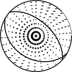
|
|
Figure 1. Waveform inversion focal mechanism
|
The best fit as a function of depth is given in the following figure:
|
|
Figure 2. Depth sensitivity for waveform mechanism
|
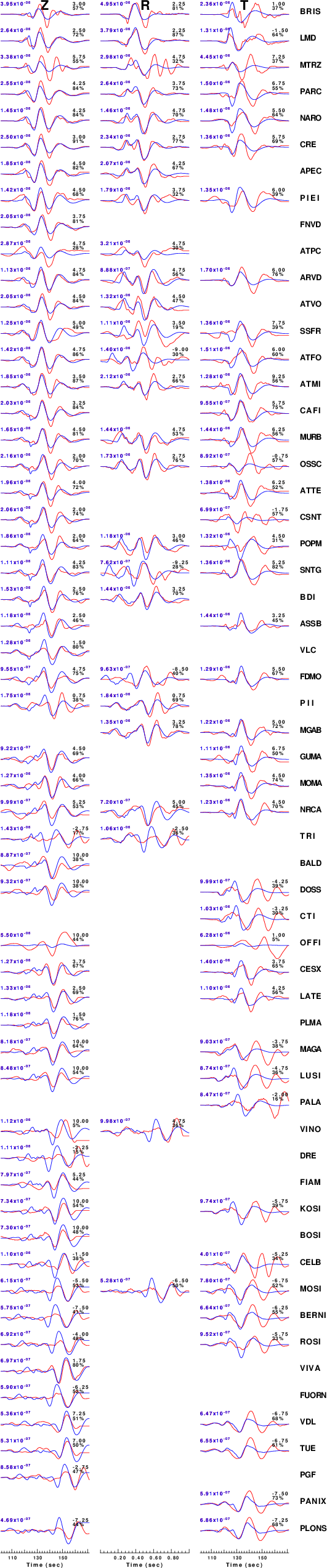
The comparison of the observed and predicted waveforms is given in the next figure. The red traces are the observed and the blue are the predicted.
Each observed-predicted component is plotted to the same scale and peak amplitudes are indicated by the numbers to the left of each trace. A pair of numbers is given in black at the right of each predicted traces. The upper number it the time shift required for maximum correlation between the observed and predicted traces. This time shift is required because the synthetics are not computed at exactly the same distance as the observed and because the velocity model used in the predictions may not be perfect.
A positive time shift indicates that the prediction is too fast and should be delayed to match the observed trace (shift to the right in this figure). A negative value indicates that the prediction is too slow. The lower number gives the percentage of variance reduction to characterize the individual goodness of fit (100% indicates a perfect fit).
The bandpass filter used in the processing and for the display was
cut o DIST/3.3 -20 o DIST/3.3 +50
rtr
taper w 0.1
hp c 0.02 n 3
lp c 0.05 n 3
|
|
Figure 3. Waveform comparison for selected depth. Red: observed; Blue - predicted. The time shift with respect to the model prediction is indicated. The percent of fit is also indicated.
|
|
|
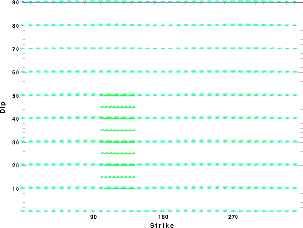
Focal mechanism sensitivity at the preferred depth. The red color indicates a very good fit to thewavefroms.
Each solution is plotted as a vector at a given value of strike and dip with the angle of the vector representing the rake angle, measured, with respect to the upward vertical (N) in the figure.
|
A check on the assumed source location is possible by looking at the time shifts between the observed and predicted traces. The time shifts for waveform matching arise for several reasons:
- The origin time and epicentral distance are incorrect
- The velocity model used for the inversion is incorrect
- The velocity model used to define the P-arrival time is not the
same as the velocity model used for the waveform inversion
(assuming that the initial trace alignment is based on the
P arrival time)
Assuming only a mislocation, the time shifts are fit to a functional form:
Time_shift = A + B cos Azimuth + C Sin Azimuth
The time shifts for this inversion lead to the next figure:
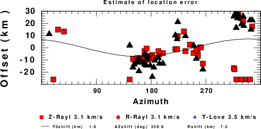
The derived shift in origin time and epicentral coordinates are given at the bottom of the figure.
Discussion
Velocity Model
The nnCIA used for the waveform synthetic seismograms and for the surface wave eigenfunctions and dispersion is as follows:
MODEL.01
C.It. A. Di Luzio et al Earth Plan Lettrs 280 (2009) 1-12 Fig 5. 7-8 MODEL/SURF3
ISOTROPIC
KGS
FLAT EARTH
1-D
CONSTANT VELOCITY
LINE08
LINE09
LINE10
LINE11
      H(KM)   VP(KM/S)   VS(KM/S) RHO(GM/CC)         QP         QS       ETAP       ETAS      FREFP      FREFS
     1.5000     3.7497     2.1436     2.2753  0.500E-02  0.100E-01   0.00       0.00       1.00       1.00
     3.0000     4.9399     2.8210     2.4858  0.500E-02  0.100E-01   0.00       0.00       1.00       1.00
     3.0000     6.0129     3.4336     2.7058  0.500E-02  0.100E-01   0.00       0.00       1.00       1.00
     7.0000     5.5516     3.1475     2.6093  0.167E-02  0.333E-02   0.00       0.00       1.00       1.00
    15.0000     5.8805     3.3583     2.6770  0.167E-02  0.333E-02   0.00       0.00       1.00       1.00
     6.0000     7.1059     4.0081     3.0002  0.167E-02  0.333E-02   0.00       0.00       1.00       1.00
     8.0000     7.1000     3.9864     3.0120  0.167E-02  0.333E-02   0.00       0.00       1.00       1.00
     0.0000     7.9000     4.4036     3.2760  0.167E-02  0.333E-02   0.00       0.00       1.00       1.00
Quality Control
Here we tabulate the reasons for not using certain digital data sets
The following stations did not have a valid response files:
DATE=Tue Jan 15 09:44:11 CST 2019
Last Changed 2019/01/14