Location
2018/04/10 03:11:30 43.07 13.04 8.0 4.6 Amatrice
Arrival Times (from USGS)
Arrival time list
Felt Map
USGS Felt map for this earthquake
USGS Felt reports page for
Focal Mechanism
 SLU Moment Tensor Solution
 ENS  2018/04/10 03:11:30:0  43.07   13.04   8.0 4.6 Amatrice

 Stations used:
   IV.AOI IV.ARVD IV.ATMI IV.CAFI IV.CASP IV.CELB IV.CERA
   IV.CERT IV.CING IV.CRE IV.CSNT IV.FIAM IV.GIUL IV.GUAR
   IV.LATE IV.LAV9 IV.LNSS IV.LPEL IV.MA9 IV.MGAB IV.MOMA
   IV.MTCE IV.OFFI IV.OSSC IV.PARC IV.PIEI IV.POFI IV.PTQR
   IV.RMP IV.SACS IV.SAMA IV.SSFR IV.TERO

 Filtering commands used:
   cut o DIST/3.3 -20 o DIST/3.3 +40
   rtr
   taper w 0.1
   hp c 0.03 n 3
   lp c 0.10 n 3

 Best Fitting Double Couple
  Mo = 9.02e+22 dyne-cm
  Mw = 4.57
  Z  = 5 km
  Plane   Strike  Dip  Rake
   NP1      160    60   -65
   NP2      297    38   -126
  Principal Axes:
   Axis    Value   Plunge  Azimuth
    T   9.02e+22     12     232
    N   0.00e+00     21     327
    P  -9.02e+22     65     116

 Moment Tensor: (dyne-cm)
    Component   Value
       Mxx     2.95e+22
       Mxy     4.80e+22
       Mxz     3.93e+21
       Myy     4.13e+22
       Myz    -4.49e+22
       Mzz    -7.08e+22


                     ##############
                 ---###################
              -----#######################
             -------------#################
           --######--------------############
          #########-----------------##########
         ##########--------------------########
        ###########----------------------#######
        ###########-----------------------######
       ############------------------------######
       #############------------------------#####
       #############------------   ----------####
       ##############----------- P -----------###
        ##############----------   -----------##
        ###############------------------------#
         ##############------------------------
          ##   ##########---------------------
           # T ###########-------------------
               ############----------------
              ###############-------------
                 ##############--------
                     ##############


 Global CMT Convention Moment Tensor:
      R          T          P
 -7.08e+22   3.93e+21   4.49e+22
  3.93e+21   2.95e+22  -4.80e+22
  4.49e+22  -4.80e+22   4.13e+22


Details of the solution is found at

http://www.eas.slu.edu/eqc/eqc_mt/MECH.IT/20180410031130/index.html
|
Preferred Solution
The preferred solution from an analysis of the surface-wave spectral amplitude radiation pattern, waveform inversion and first motion observations is
      STK = 160
      DIP = 60
     RAKE = -65
       MW = 4.57
       HS = 5.0
The NDK file is 20180410031130.ndk
The waveform inversion is preferred.
Moment Tensor Comparison
The following compares this source inversion to others
| SLU |
INGVTDMT |
 SLU Moment Tensor Solution
 ENS  2018/04/10 03:11:30:0  43.07   13.04   8.0 4.6 Amatrice

 Stations used:
   IV.AOI IV.ARVD IV.ATMI IV.CAFI IV.CASP IV.CELB IV.CERA
   IV.CERT IV.CING IV.CRE IV.CSNT IV.FIAM IV.GIUL IV.GUAR
   IV.LATE IV.LAV9 IV.LNSS IV.LPEL IV.MA9 IV.MGAB IV.MOMA
   IV.MTCE IV.OFFI IV.OSSC IV.PARC IV.PIEI IV.POFI IV.PTQR
   IV.RMP IV.SACS IV.SAMA IV.SSFR IV.TERO

 Filtering commands used:
   cut o DIST/3.3 -20 o DIST/3.3 +40
   rtr
   taper w 0.1
   hp c 0.03 n 3
   lp c 0.10 n 3

 Best Fitting Double Couple
  Mo = 9.02e+22 dyne-cm
  Mw = 4.57
  Z  = 5 km
  Plane   Strike  Dip  Rake
   NP1      160    60   -65
   NP2      297    38   -126
  Principal Axes:
   Axis    Value   Plunge  Azimuth
    T   9.02e+22     12     232
    N   0.00e+00     21     327
    P  -9.02e+22     65     116

 Moment Tensor: (dyne-cm)
    Component   Value
       Mxx     2.95e+22
       Mxy     4.80e+22
       Mxz     3.93e+21
       Myy     4.13e+22
       Myz    -4.49e+22
       Mzz    -7.08e+22


                     ##############
                 ---###################
              -----#######################
             -------------#################
           --######--------------############
          #########-----------------##########
         ##########--------------------########
        ###########----------------------#######
        ###########-----------------------######
       ############------------------------######
       #############------------------------#####
       #############------------   ----------####
       ##############----------- P -----------###
        ##############----------   -----------##
        ###############------------------------#
         ##############------------------------
          ##   ##########---------------------
           # T ###########-------------------
               ############----------------
              ###############-------------
                 ##############--------
                     ##############


 Global CMT Convention Moment Tensor:
      R          T          P
 -7.08e+22   3.93e+21   4.49e+22
  3.93e+21   2.95e+22  -4.80e+22
  4.49e+22  -4.80e+22   4.13e+22


Details of the solution is found at

http://www.eas.slu.edu/eqc/eqc_mt/MECH.IT/20180410031130/index.html
|
|
Magnitudes
ML Magnitude
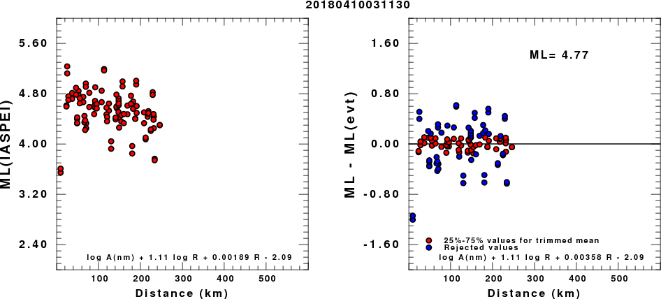
(a) ML computed using the IASPEI formula for Horizontal components; (b) ML residuals computed using a modified IASPEI formula that accounts for path specific attenuation; the values used for the trimmed mean are indicated. The ML relation used for each figure is given at the bottom of each plot.
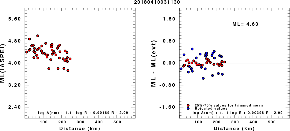
(a) ML computed using the IASPEI formula for Vertical components (research); (b) ML residuals computed using a modified IASPEI formula that accounts for path specific attenuation; the values used for the trimmed mean are indicated. The ML relation used for each figure is given at the bottom of each plot.
Waveform Inversion
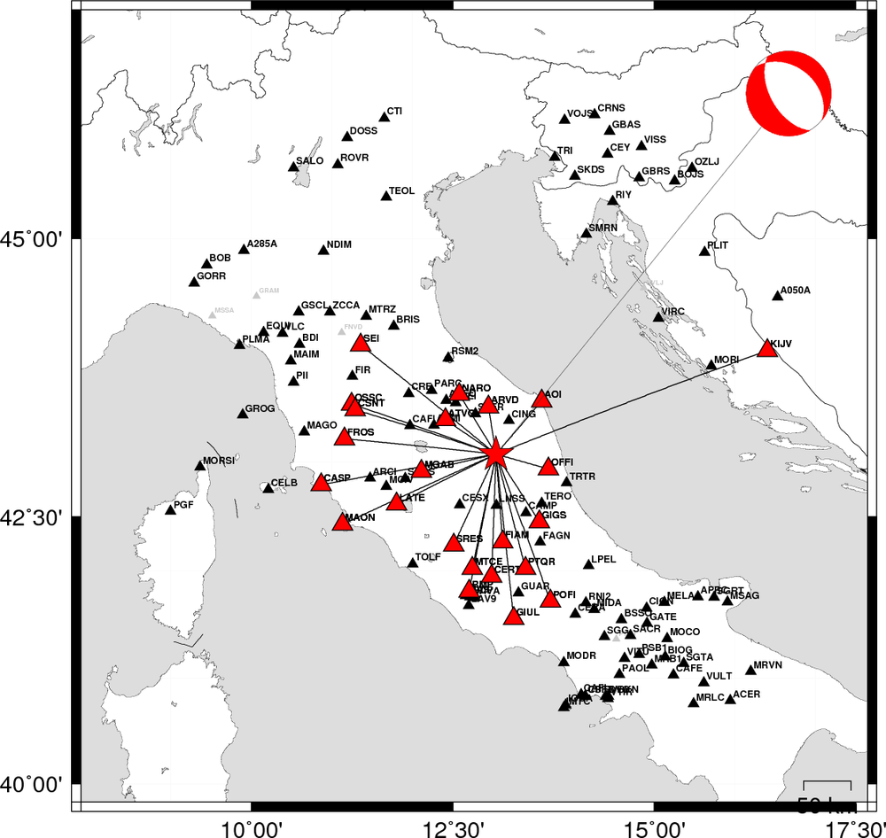
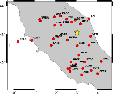
The focal mechanism was determined using broadband seismic waveforms. The location of the event and the
and stations used for the waveform inversion are shown in the next figure.
|
|
Location of broadband stations used for waveform inversion
|
The program wvfgrd96 was used with good traces observed at short distance to determine the focal mechanism, depth and seismic moment. This technique requires a high quality signal and well determined velocity model for the Green functions. To the extent that these are the quality data, this type of mechanism should be preferred over the radiation pattern technique which requires the separate step of defining the pressure and tension quadrants and the correct strike.
The observed and predicted traces are filtered using the following gsac commands:
cut o DIST/3.3 -20 o DIST/3.3 +40
rtr
taper w 0.1
hp c 0.03 n 3
lp c 0.10 n 3
The results of this grid search from 0.5 to 19 km depth are as follow:
           DEPTH  STK   DIP  RAKE   MW    FIT
WVFGRD96    1.0   175    65   -45   4.32 0.4500
WVFGRD96    2.0   175    75   -55   4.42 0.5101
WVFGRD96    3.0   170    70   -55   4.44 0.5784
WVFGRD96    4.0   160    60   -65   4.49 0.6180
WVFGRD96    5.0   160    60   -65   4.57 0.6551
WVFGRD96    6.0   160    60   -65   4.57 0.6481
WVFGRD96    7.0   170    65   -55   4.54 0.6151
WVFGRD96    8.0   180    75   -35   4.50 0.5734
WVFGRD96    9.0   180    80   -35   4.50 0.5524
WVFGRD96   10.0   180    80   -35   4.51 0.5306
WVFGRD96   11.0   180    80   -35   4.52 0.5086
WVFGRD96   12.0   180    80   -35   4.53 0.4854
WVFGRD96   13.0   185    90   -30   4.53 0.4624
WVFGRD96   14.0     5    85    30   4.54 0.4398
WVFGRD96   15.0     5    75   -25   4.57 0.4218
WVFGRD96   16.0     5    75   -25   4.58 0.4092
WVFGRD96   17.0     5    75   -25   4.59 0.3963
WVFGRD96   18.0     5    75   -25   4.60 0.3828
WVFGRD96   19.0     5    75   -25   4.60 0.3689
The best solution is
WVFGRD96 5.0 160 60 -65 4.57 0.6551
The mechanism correspond to the best fit is
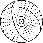
|
|
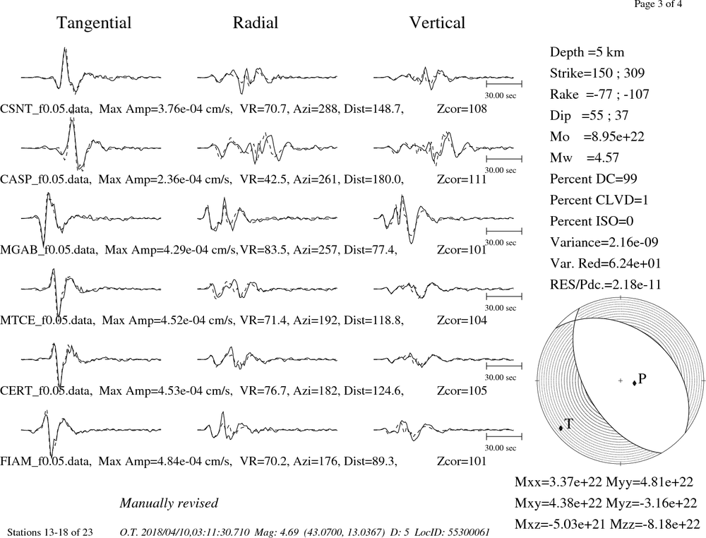
Figure 1. Waveform inversion focal mechanism
|
The best fit as a function of depth is given in the following figure:
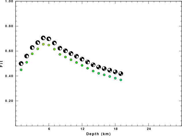
|
|
Figure 2. Depth sensitivity for waveform mechanism
|
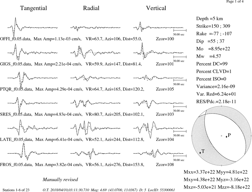
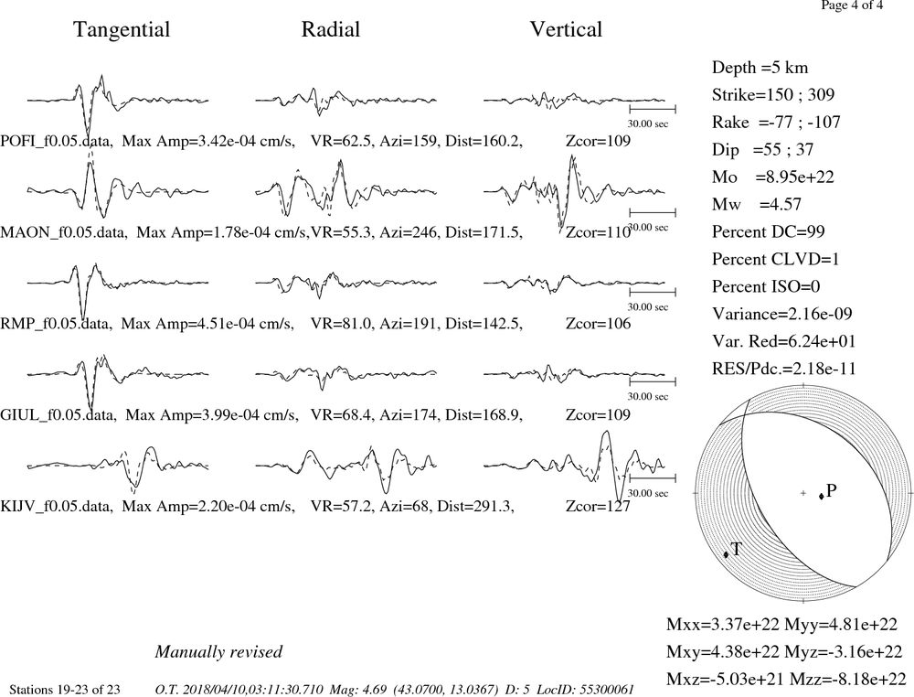
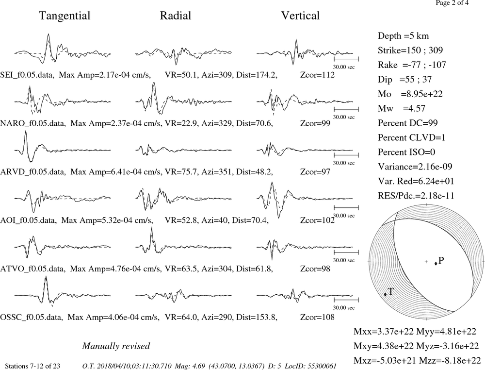
The comparison of the observed and predicted waveforms is given in the next figure. The red traces are the observed and the blue are the predicted.
Each observed-predicted component is plotted to the same scale and peak amplitudes are indicated by the numbers to the left of each trace. A pair of numbers is given in black at the right of each predicted traces. The upper number it the time shift required for maximum correlation between the observed and predicted traces. This time shift is required because the synthetics are not computed at exactly the same distance as the observed and because the velocity model used in the predictions may not be perfect.
A positive time shift indicates that the prediction is too fast and should be delayed to match the observed trace (shift to the right in this figure). A negative value indicates that the prediction is too slow. The lower number gives the percentage of variance reduction to characterize the individual goodness of fit (100% indicates a perfect fit).
The bandpass filter used in the processing and for the display was
cut o DIST/3.3 -20 o DIST/3.3 +40
rtr
taper w 0.1
hp c 0.03 n 3
lp c 0.10 n 3
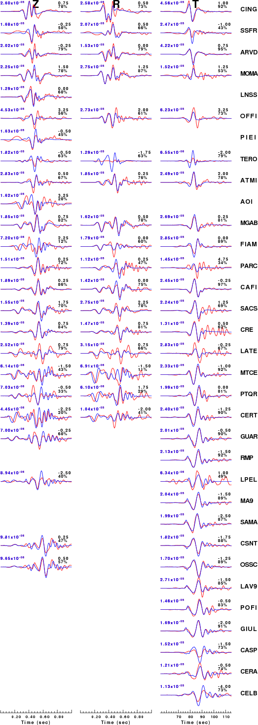
|
|
Figure 3. Waveform comparison for selected depth. Red: observed; Blue - predicted. The time shift with respect to the model prediction is indicated. The percent of fit is also indicated.
|
|
|
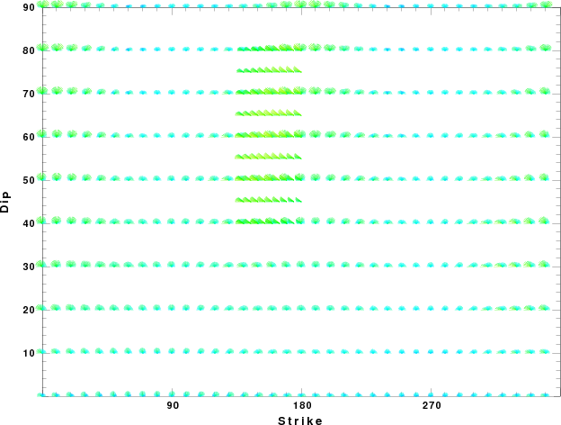
Focal mechanism sensitivity at the preferred depth. The red color indicates a very good fit to thewavefroms.
Each solution is plotted as a vector at a given value of strike and dip with the angle of the vector representing the rake angle, measured, with respect to the upward vertical (N) in the figure.
|
A check on the assumed source location is possible by looking at the time shifts between the observed and predicted traces. The time shifts for waveform matching arise for several reasons:
- The origin time and epicentral distance are incorrect
- The velocity model used for the inversion is incorrect
- The velocity model used to define the P-arrival time is not the
same as the velocity model used for the waveform inversion
(assuming that the initial trace alignment is based on the
P arrival time)
Assuming only a mislocation, the time shifts are fit to a functional form:
Time_shift = A + B cos Azimuth + C Sin Azimuth
The time shifts for this inversion lead to the next figure:
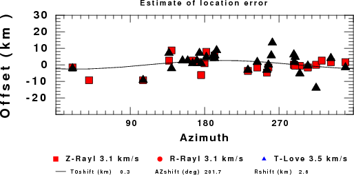
The derived shift in origin time and epicentral coordinates are given at the bottom of the figure.
Discussion
Velocity Model
The nnCIA used for the waveform synthetic seismograms and for the surface wave eigenfunctions and dispersion is as follows:
MODEL.01
C.It. A. Di Luzio et al Earth Plan Lettrs 280 (2009) 1-12 Fig 5. 7-8 MODEL/SURF3
ISOTROPIC
KGS
FLAT EARTH
1-D
CONSTANT VELOCITY
LINE08
LINE09
LINE10
LINE11
      H(KM)   VP(KM/S)   VS(KM/S) RHO(GM/CC)         QP         QS       ETAP       ETAS      FREFP      FREFS
     1.5000     3.7497     2.1436     2.2753  0.500E-02  0.100E-01   0.00       0.00       1.00       1.00
     3.0000     4.9399     2.8210     2.4858  0.500E-02  0.100E-01   0.00       0.00       1.00       1.00
     3.0000     6.0129     3.4336     2.7058  0.500E-02  0.100E-01   0.00       0.00       1.00       1.00
     7.0000     5.5516     3.1475     2.6093  0.167E-02  0.333E-02   0.00       0.00       1.00       1.00
    15.0000     5.8805     3.3583     2.6770  0.167E-02  0.333E-02   0.00       0.00       1.00       1.00
     6.0000     7.1059     4.0081     3.0002  0.167E-02  0.333E-02   0.00       0.00       1.00       1.00
     8.0000     7.1000     3.9864     3.0120  0.167E-02  0.333E-02   0.00       0.00       1.00       1.00
     0.0000     7.9000     4.4036     3.2760  0.167E-02  0.333E-02   0.00       0.00       1.00       1.00
Quality Control
Here we tabulate the reasons for not using certain digital data sets
The following stations did not have a valid response files:
DATE=Tue Apr 10 08:17:47 CDT 2018
Last Changed 2018/04/10