Location

2016/10/26 19:18:05 42.9150 13.1280 8.4 5.90

SLU Moment Tensor Solution ENS 2016/10/26 19:18:05:9 42.92 13.13 8.4 5.9 Stations used: IV.CERT IV.CRE IV.FIAM IV.GUAR IV.LPEL IV.MCIV IV.MGAB IV.MTCE IV.PTQR IV.RMP IV.SACS IV.SRES IV.TOLF MN.AQU Filtering commands used: cut o DIST/3.3 -20 o DIST/3.3 +70 rtr taper w 0.1 hp c 0.01 n 3 lp c 0.05 n 3 Best Fitting Double Couple Mo = 8.04e+24 dyne-cm Mw = 5.87 Z = 5 km Plane Strike Dip Rake NP1 162 45 -85 NP2 335 45 -95 Principal Axes: Axis Value Plunge Azimuth T 8.04e+24 0 249 N 0.00e+00 4 339 P -8.04e+24 86 157 Moment Tensor: (dyne-cm) Component Value Mxx 1.05e+24 Mxy 2.75e+24 Mxz 4.49e+23 Myy 6.95e+24 Myz -2.09e+23 Mzz -8.00e+24 ############## ###-----############## #####----------############# #####-------------############ ######----------------############ #######------------------########### #######--------------------########### ########---------------------########### ########----------------------########## #########-----------------------########## #########----------- ----------######### ##########---------- P ----------######### ##########---------- ----------######### ########-----------------------####### T #########----------------------####### #########----------------------###### ###########-------------------###### ###########------------------##### ###########----------------### ############-------------### ###########----------# ############-- Global CMT Convention Moment Tensor: R T P -8.00e+24 4.49e+23 2.09e+23 4.49e+23 1.05e+24 -2.75e+24 2.09e+23 -2.75e+24 6.95e+24 Details of the solution is found at http://www.eas.slu.edu/eqc/eqc_mt/MECH.IT/20161026191805/index.html

Preferred Solution

      STK = 335
      DIP = 45
     RAKE = -95
       MW = 5.87
       HS = 5.0

The waveform inversion is preferred.

Moment Tensor Comparison

The following compares this source inversion to others

SLU	GCMT	USGSW
SLU Moment Tensor Solution ENS 2016/10/26 19:18:05:9 42.92 13.13 8.4 5.9 Stations used: IV.CERT IV.CRE IV.FIAM IV.GUAR IV.LPEL IV.MCIV IV.MGAB IV.MTCE IV.PTQR IV.RMP IV.SACS IV.SRES IV.TOLF MN.AQU Filtering commands used: cut o DIST/3.3 -20 o DIST/3.3 +70 rtr taper w 0.1 hp c 0.01 n 3 lp c 0.05 n 3 Best Fitting Double Couple Mo = 8.04e+24 dyne-cm Mw = 5.87 Z = 5 km Plane Strike Dip Rake NP1 162 45 -85 NP2 335 45 -95 Principal Axes: Axis Value Plunge Azimuth T 8.04e+24 0 249 N 0.00e+00 4 339 P -8.04e+24 86 157 Moment Tensor: (dyne-cm) Component Value Mxx 1.05e+24 Mxy 2.75e+24 Mxz 4.49e+23 Myy 6.95e+24 Myz -2.09e+23 Mzz -8.00e+24 ############## ###-----############## #####----------############# #####-------------############ ######----------------############ #######------------------########### #######--------------------########### ########---------------------########### ########----------------------########## #########-----------------------########## #########----------- ----------######### ##########---------- P ----------######### ##########---------- ----------######### ########-----------------------####### T #########----------------------####### #########----------------------###### ###########-------------------###### ###########------------------##### ###########----------------### ############-------------### ###########----------# ############-- Global CMT Convention Moment Tensor: R T P -8.00e+24 4.49e+23 2.09e+23 4.49e+23 1.05e+24 -2.75e+24 2.09e+23 -2.75e+24 6.95e+24 Details of the solution is found at http://www.eas.slu.edu/eqc/eqc_mt/MECH.IT/20161026191805/index.html	October 26, 2016, CENTRAL ITALY, MW=6.1 Howard Koss CENTROID-MOMENT-TENSOR SOLUTION GCMT EVENT: C201610261918A DATA: II IU CU G IC LD DK GE KP MN L.P.BODY WAVES: 88S, 181C, T= 40 MANTLE WAVES: 72S, 97C, T=125 SURFACE WAVES: 111S, 270C, T= 50 TIMESTAMP: Q-20161026204735 CENTROID LOCATION: ORIGIN TIME: 19:18:12.4 0.1 LAT:42.88N 0.01;LON: 13.11E 0.00 DEP: 12.0 FIX;TRIANG HDUR: 2.7 MOMENT TENSOR: SCALE 10**25 D-CM RR=-1.630 0.011; TT= 0.283 0.011 PP= 1.350 0.010; RT=-0.107 0.035 RP=-0.522 0.031; TP=-0.722 0.010 PRINCIPAL AXES: 1.(T) VAL= 1.767;PLG= 7;AZM= 65 2.(N) -0.017; 11; 156 3.(P) -1.746; 77; 302 BEST DBLE.COUPLE:M0= 1.76*10**25 NP1: STRIKE=142;DIP=39;SLIP=-107 NP2: STRIKE=344;DIP=53;SLIP= -76 --######### ---------########## #------------########## ##---------------########## ###----------------######## ###------------------####### T ###-------------------###### #####-------- -------########## #####-------- P --------######### ######------- --------######### ######------------------######### ######------------------####### ########----------------####### ########--------------####### ##########-----------###### ###########-------##### ###############---- ##########-	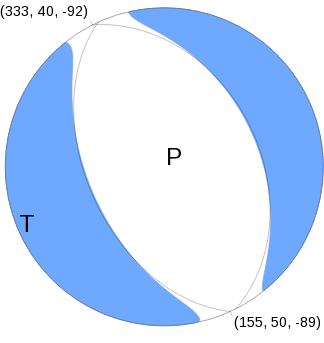W-phase Moment Tensor (Mww) Moment 1.840e+18 N-m Magnitude 6.1 Mww Depth 11.5 km Percent DC 90 % Half Duration 4 s Catalog US Data Source US1 Contributor US1 Nodal Planes Plane Strike Dip Rake NP1 333 40 -92 NP2 155 50 -89 Principal Axes Axis Value Plunge Azimuth T 1.885e+18 N-m 5 244 N -0.092e+18 N-m 1 335 P -1.793e+18 N-m 85 78

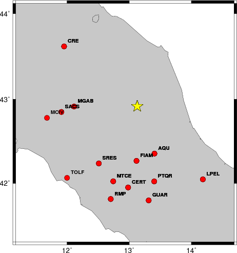
Waveform Inversion

The focal mechanism was determined using broadband seismic waveforms. The location of the event and the and stations used for the waveform inversion are shown in the next figure.

Location of broadband stations used for waveform inversion

The program wvfgrd96 was used with good traces observed at short distance to determine the focal mechanism, depth and seismic moment. This technique requires a high quality signal and well determined velocity model for the Green functions. To the extent that these are the quality data, this type of mechanism should be preferred over the radiation pattern technique which requires the separate step of defining the pressure and tension quadrants and the correct strike.

The observed and predicted traces are filtered using the following gsac commands:

cut o DIST/3.3 -20 o DIST/3.3 +70
rtr
taper w 0.1
hp c 0.01 n 3 
lp c 0.05 n 3 

           DEPTH  STK   DIP  RAKE   MW    FIT
WVFGRD96    1.0   170    50   -70   5.67 0.6129
WVFGRD96    2.0   165    50   -80   5.74 0.6987
WVFGRD96    3.0   160    45   -85   5.79 0.7512
WVFGRD96    4.0   160    45   -85   5.83 0.7415
WVFGRD96    5.0   335    45   -95   5.87 0.7812
WVFGRD96    6.0   160    50   -85   5.86 0.6740
WVFGRD96    7.0   355    45   -60   5.80 0.5409
WVFGRD96    8.0   200    85   -25   5.70 0.5005
WVFGRD96    9.0    20    90    25   5.71 0.4924
WVFGRD96   10.0   200    70    25   5.71 0.4967
WVFGRD96   11.0   200    65    20   5.72 0.5014
WVFGRD96   12.0   200    70    25   5.73 0.5074
WVFGRD96   13.0   200    70    25   5.74 0.5156
WVFGRD96   14.0   200    70    25   5.75 0.5238
WVFGRD96   15.0   200    70    30   5.76 0.5175

The best solution is

WVFGRD96    5.0   335    45   -95   5.87 0.7812

The mechanism correspond to the best fit is

Figure 1. Waveform inversion focal mechanism

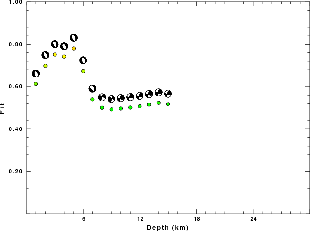
The best fit as a function of depth is given in the following figure:

Figure 2. Depth sensitivity for waveform mechanism

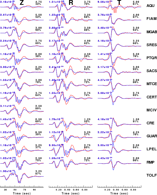
The comparison of the observed and predicted waveforms is given in the next figure. The red traces are the observed and the blue are the predicted. Each observed-predicted component is plotted to the same scale and peak amplitudes are indicated by the numbers to the left of each trace. A pair of numbers is given in black at the right of each predicted traces. The upper number it the time shift required for maximum correlation between the observed and predicted traces. This time shift is required because the synthetics are not computed at exactly the same distance as the observed and because the velocity model used in the predictions may not be perfect. A positive time shift indicates that the prediction is too fast and should be delayed to match the observed trace (shift to the right in this figure). A negative value indicates that the prediction is too slow. The lower number gives the percentage of variance reduction to characterize the individual goodness of fit (100% indicates a perfect fit).

The bandpass filter used in the processing and for the display was

cut o DIST/3.3 -20 o DIST/3.3 +70
rtr
taper w 0.1
hp c 0.01 n 3 
lp c 0.05 n 3 

Figure 3. Waveform comparison for selected depth. Red: observed; Blue - predicted. The time shift with respect to the model prediction is indicated. The percent of fit is also indicated.

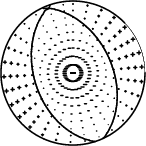
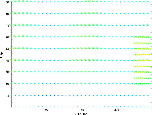
Focal mechanism sensitivity at the preferred depth. The red color indicates a very good fit to thewavefroms. Each solution is plotted as a vector at a given value of strike and dip with the angle of the vector representing the rake angle, measured, with respect to the upward vertical (N) in the figure.

Discussion

Velocity Model

The nnCIA used for the waveform synthetic seismograms and for the surface wave eigenfunctions and dispersion is as follows:

MODEL.01
C.It. A. Di Luzio et al Earth Plan Lettrs 280 (2009) 1-12 Fig 5. 7-8 MODEL/SURF3
ISOTROPIC
KGS
FLAT EARTH
1-D
CONSTANT VELOCITY
LINE08
LINE09
LINE10
LINE11
      H(KM)   VP(KM/S)   VS(KM/S) RHO(GM/CC)         QP         QS       ETAP       ETAS      FREFP      FREFS
     1.5000     3.7497     2.1436     2.2753  0.500E-02  0.100E-01   0.00       0.00       1.00       1.00    
     3.0000     4.9399     2.8210     2.4858  0.500E-02  0.100E-01   0.00       0.00       1.00       1.00    
     3.0000     6.0129     3.4336     2.7058  0.500E-02  0.100E-01   0.00       0.00       1.00       1.00    
     7.0000     5.5516     3.1475     2.6093  0.167E-02  0.333E-02   0.00       0.00       1.00       1.00    
    15.0000     5.8805     3.3583     2.6770  0.167E-02  0.333E-02   0.00       0.00       1.00       1.00    
     6.0000     7.1059     4.0081     3.0002  0.167E-02  0.333E-02   0.00       0.00       1.00       1.00    
     8.0000     7.1000     3.9864     3.0120  0.167E-02  0.333E-02   0.00       0.00       1.00       1.00    
     0.0000     7.9000     4.4036     3.2760  0.167E-02  0.333E-02   0.00       0.00       1.00       1.00    

Quality Control

Here we tabulate the reasons for not using certain digital data sets

The following stations did not have a valid response files:

DATE=Wed Oct 26 20:48:21 CDT 2016