Location
2014/12/28 21:43:38 39.292 16.358 11.1 4.4 Italy
Arrival Times (from USGS)
Arrival time list
Felt Map
USGS Felt map for this earthquake
USGS Felt reports page for
Focal Mechanism
 SLU Moment Tensor Solution
 ENS  2014/12/28 21:43:38:0  39.29   16.36  11.1 4.4 Italy

 Stations used:
   IV.CMPR IV.JOPP IV.MCEL IV.MCRV IV.MGR IV.MRLC IV.PALZ
   IV.SALB IV.SERS MN.TIP

 Filtering commands used:
   cut o DIST/3.3 -30 o DIST/3.3 +70
   rtr
   taper w 0.1
   hp c 0.02 n 3
   lp c 0.06 n 3

 Best Fitting Double Couple
  Mo = 3.55e+22 dyne-cm
  Mw = 4.30
  Z  = 15 km
  Plane   Strike  Dip  Rake
   NP1      220    55   -45
   NP2      340    55   -135
  Principal Axes:
   Axis    Value   Plunge  Azimuth
    T   3.55e+22      0     280
    N   0.00e+00     35      10
    P  -3.55e+22     55     190

 Moment Tensor: (dyne-cm)
    Component   Value
       Mxx    -1.05e+22
       Mxy    -8.04e+21
       Mxz     1.65e+22
       Myy     3.41e+22
       Myz     2.68e+21
       Mzz    -2.36e+22


                     --------------
                 ########--------------
              ##############---------#####
             #################--###########
           #################---##############
          ################-------#############
         ###############----------#############
        ##############-------------#############
         ###########----------------############
       T ##########-----------------#############
         #########-------------------############
       ##########---------------------###########
       #########----------------------###########
        #######-----------------------##########
        #######----------   ----------##########
         #####----------- P ----------#########
          ####-----------   ----------########
           ###------------------------#######
             #------------------------#####
              #----------------------#####
                 -------------------###
                     --------------


 Global CMT Convention Moment Tensor:
      R          T          P
 -2.36e+22   1.65e+22  -2.68e+21
  1.65e+22  -1.05e+22   8.04e+21
 -2.68e+21   8.04e+21   3.41e+22


Details of the solution is found at

http://www.eas.slu.edu/eqc/eqc_mt/MECH.IT/20141228214338/index.html
|
Preferred Solution
The preferred solution from an analysis of the surface-wave spectral amplitude radiation pattern, waveform inversion and first motion observations is
      STK = 220
      DIP = 55
     RAKE = -45
       MW = 4.30
       HS = 15.0
The NDK file is 20141228214338.ndk
The waveform inversion is preferred.
Moment Tensor Comparison
The following compares this source inversion to others
| SLU |
INGVTDMT |
 SLU Moment Tensor Solution
 ENS  2014/12/28 21:43:38:0  39.29   16.36  11.1 4.4 Italy

 Stations used:
   IV.CMPR IV.JOPP IV.MCEL IV.MCRV IV.MGR IV.MRLC IV.PALZ
   IV.SALB IV.SERS MN.TIP

 Filtering commands used:
   cut o DIST/3.3 -30 o DIST/3.3 +70
   rtr
   taper w 0.1
   hp c 0.02 n 3
   lp c 0.06 n 3

 Best Fitting Double Couple
  Mo = 3.55e+22 dyne-cm
  Mw = 4.30
  Z  = 15 km
  Plane   Strike  Dip  Rake
   NP1      220    55   -45
   NP2      340    55   -135
  Principal Axes:
   Axis    Value   Plunge  Azimuth
    T   3.55e+22      0     280
    N   0.00e+00     35      10
    P  -3.55e+22     55     190

 Moment Tensor: (dyne-cm)
    Component   Value
       Mxx    -1.05e+22
       Mxy    -8.04e+21
       Mxz     1.65e+22
       Myy     3.41e+22
       Myz     2.68e+21
       Mzz    -2.36e+22


                     --------------
                 ########--------------
              ##############---------#####
             #################--###########
           #################---##############
          ################-------#############
         ###############----------#############
        ##############-------------#############
         ###########----------------############
       T ##########-----------------#############
         #########-------------------############
       ##########---------------------###########
       #########----------------------###########
        #######-----------------------##########
        #######----------   ----------##########
         #####----------- P ----------#########
          ####-----------   ----------########
           ###------------------------#######
             #------------------------#####
              #----------------------#####
                 -------------------###
                     --------------


 Global CMT Convention Moment Tensor:
      R          T          P
 -2.36e+22   1.65e+22  -2.68e+21
  1.65e+22  -1.05e+22   8.04e+21
 -2.68e+21   8.04e+21   3.41e+22


Details of the solution is found at

http://www.eas.slu.edu/eqc/eqc_mt/MECH.IT/20141228214338/index.html
|
|
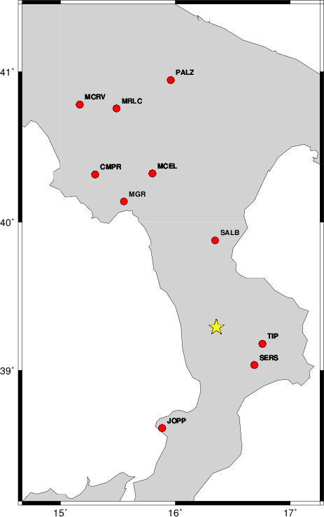
Waveform Inversion
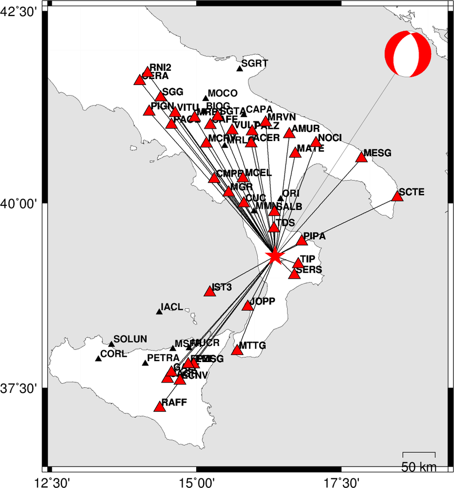
The focal mechanism was determined using broadband seismic waveforms. The location of the event and the
and stations used for the waveform inversion are shown in the next figure.
|
|
Location of broadband stations used for waveform inversion
|
The program wvfgrd96 was used with good traces observed at short distance to determine the focal mechanism, depth and seismic moment. This technique requires a high quality signal and well determined velocity model for the Green functions. To the extent that these are the quality data, this type of mechanism should be preferred over the radiation pattern technique which requires the separate step of defining the pressure and tension quadrants and the correct strike.
The observed and predicted traces are filtered using the following gsac commands:
cut o DIST/3.3 -30 o DIST/3.3 +70
rtr
taper w 0.1
hp c 0.02 n 3
lp c 0.06 n 3
The results of this grid search from 0.5 to 19 km depth are as follow:
           DEPTH  STK   DIP  RAKE   MW    FIT
WVFGRD96    1.0   190    50   -85   4.08 0.3904
WVFGRD96    2.0    65    90    50   4.15 0.4304
WVFGRD96    3.0   235    80   -50   4.15 0.4846
WVFGRD96    4.0   230    75   -45   4.15 0.5238
WVFGRD96    5.0   230    75   -50   4.21 0.5592
WVFGRD96    6.0   225    65   -50   4.22 0.5905
WVFGRD96    7.0     5    45  -100   4.29 0.6309
WVFGRD96    8.0   205    45   -70   4.28 0.6607
WVFGRD96    9.0   205    45   -70   4.28 0.6874
WVFGRD96   10.0   205    45   -70   4.28 0.6995
WVFGRD96   11.0   210    45   -60   4.28 0.7020
WVFGRD96   12.0   215    50   -55   4.27 0.7036
WVFGRD96   13.0   215    50   -55   4.28 0.7007
WVFGRD96   14.0   225    55   -40   4.28 0.6960
WVFGRD96   15.0   220    55   -45   4.30 0.7060
WVFGRD96   16.0   220    55   -45   4.31 0.7005
WVFGRD96   17.0   225    60   -40   4.31 0.6950
WVFGRD96   18.0   230    70   -35   4.30 0.6876
WVFGRD96   19.0   230    70   -30   4.31 0.6827
WVFGRD96   20.0   230    75   -30   4.31 0.6774
WVFGRD96   21.0   230    75   -30   4.32 0.6713
WVFGRD96   22.0   230    75   -30   4.33 0.6643
WVFGRD96   23.0   235    85   -30   4.33 0.6567
WVFGRD96   24.0   235    85   -30   4.33 0.6486
WVFGRD96   25.0   235    85   -30   4.34 0.6398
WVFGRD96   26.0   235    85   -30   4.35 0.6293
WVFGRD96   27.0   235    85   -30   4.36 0.6191
WVFGRD96   28.0   235    85   -30   4.37 0.6082
WVFGRD96   29.0   235    85   -25   4.40 0.5978
The best solution is
WVFGRD96 15.0 220 55 -45 4.30 0.7060
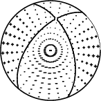
The mechanism correspond to the best fit is
|
|
Figure 1. Waveform inversion focal mechanism
|
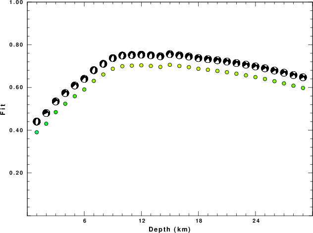
The best fit as a function of depth is given in the following figure:
|
|
Figure 2. Depth sensitivity for waveform mechanism
|
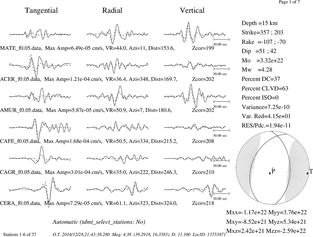
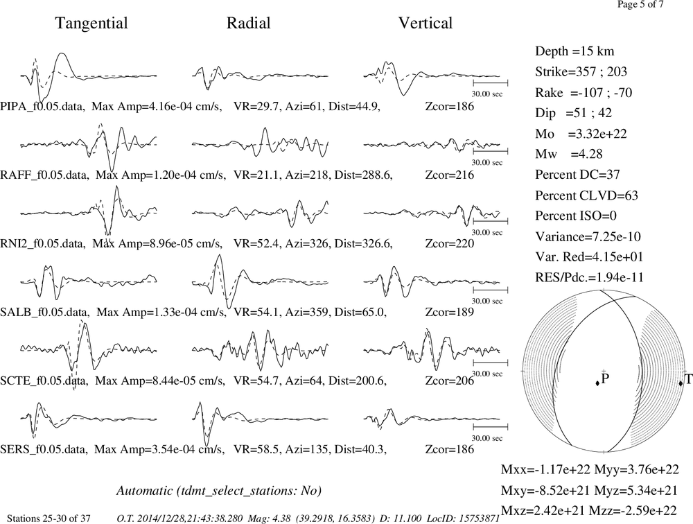
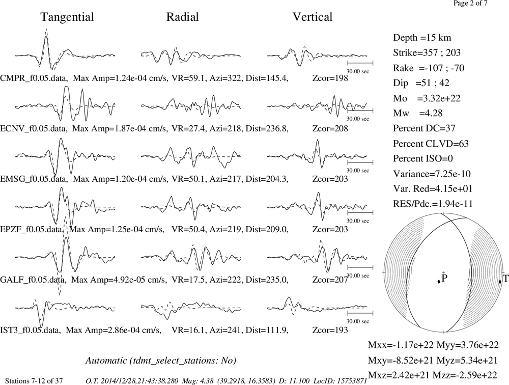
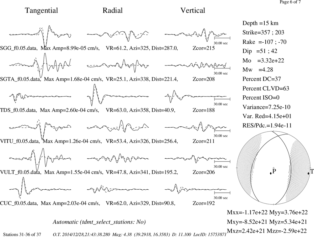
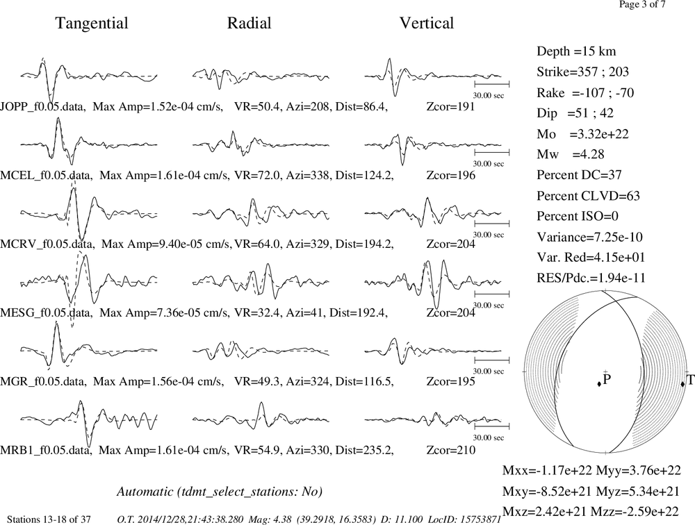
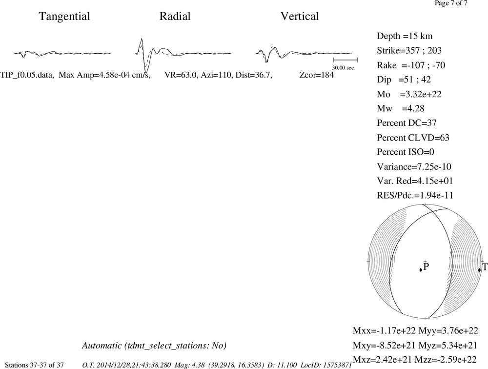
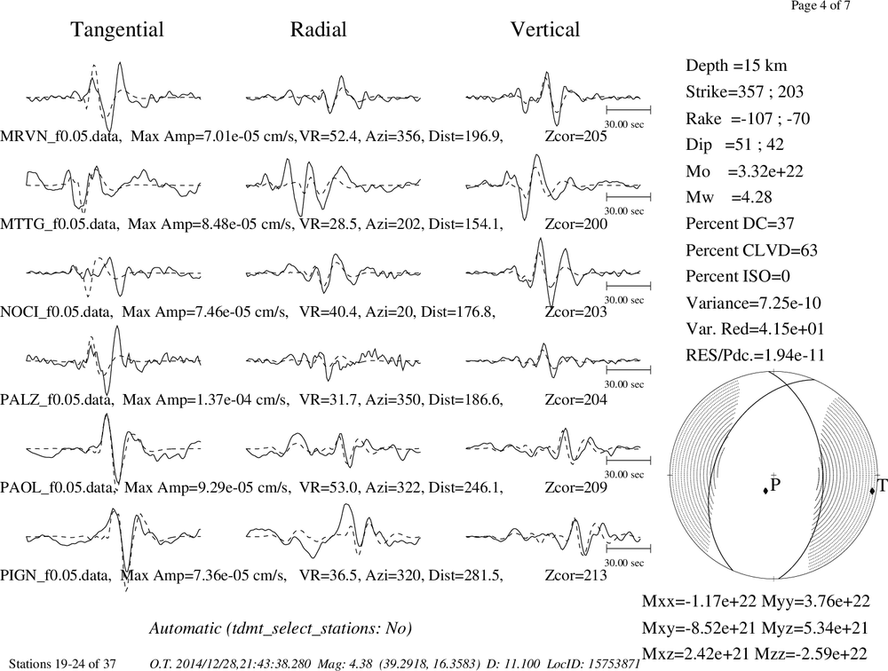
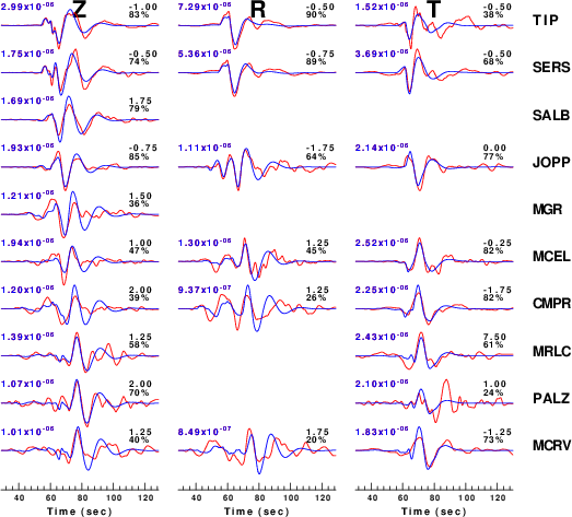
The comparison of the observed and predicted waveforms is given in the next figure. The red traces are the observed and the blue are the predicted.
Each observed-predicted component is plotted to the same scale and peak amplitudes are indicated by the numbers to the left of each trace. A pair of numbers is given in black at the right of each predicted traces. The upper number it the time shift required for maximum correlation between the observed and predicted traces. This time shift is required because the synthetics are not computed at exactly the same distance as the observed and because the velocity model used in the predictions may not be perfect.
A positive time shift indicates that the prediction is too fast and should be delayed to match the observed trace (shift to the right in this figure). A negative value indicates that the prediction is too slow. The lower number gives the percentage of variance reduction to characterize the individual goodness of fit (100% indicates a perfect fit).
The bandpass filter used in the processing and for the display was
cut o DIST/3.3 -30 o DIST/3.3 +70
rtr
taper w 0.1
hp c 0.02 n 3
lp c 0.06 n 3
|
|
Figure 3. Waveform comparison for selected depth. Red: observed; Blue - predicted. The time shift with respect to the model prediction is indicated. The percent of fit is also indicated.
|
|
|
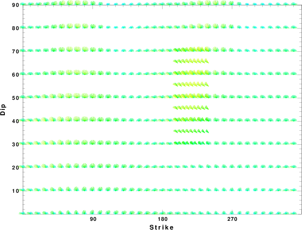
Focal mechanism sensitivity at the preferred depth. The red color indicates a very good fit to thewavefroms.
Each solution is plotted as a vector at a given value of strike and dip with the angle of the vector representing the rake angle, measured, with respect to the upward vertical (N) in the figure.
|
A check on the assumed source location is possible by looking at the time shifts between the observed and predicted traces. The time shifts for waveform matching arise for several reasons:
- The origin time and epicentral distance are incorrect
- The velocity model used for the inversion is incorrect
- The velocity model used to define the P-arrival time is not the
same as the velocity model used for the waveform inversion
(assuming that the initial trace alignment is based on the
P arrival time)
Assuming only a mislocation, the time shifts are fit to a functional form:
Time_shift = A + B cos Azimuth + C Sin Azimuth
The time shifts for this inversion lead to the next figure:
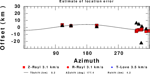
The derived shift in origin time and epicentral coordinates are given at the bottom of the figure.
Discussion
Velocity Model
The nnCIA used for the waveform synthetic seismograms and for the surface wave eigenfunctions and dispersion is as follows:
MODEL.01
C.It. A. Di Luzio et al Earth Plan Lettrs 280 (2009) 1-12 Fig 5. 7-8 MODEL/SURF3
ISOTROPIC
KGS
FLAT EARTH
1-D
CONSTANT VELOCITY
LINE08
LINE09
LINE10
LINE11
      H(KM)   VP(KM/S)   VS(KM/S) RHO(GM/CC)         QP         QS       ETAP       ETAS      FREFP      FREFS
     1.5000     3.7497     2.1436     2.2753  0.500E-02  0.100E-01   0.00       0.00       1.00       1.00
     3.0000     4.9399     2.8210     2.4858  0.500E-02  0.100E-01   0.00       0.00       1.00       1.00
     3.0000     6.0129     3.4336     2.7058  0.500E-02  0.100E-01   0.00       0.00       1.00       1.00
     7.0000     5.5516     3.1475     2.6093  0.167E-02  0.333E-02   0.00       0.00       1.00       1.00
    15.0000     5.8805     3.3583     2.6770  0.167E-02  0.333E-02   0.00       0.00       1.00       1.00
     6.0000     7.1059     4.0081     3.0002  0.167E-02  0.333E-02   0.00       0.00       1.00       1.00
     8.0000     7.1000     3.9864     3.0120  0.167E-02  0.333E-02   0.00       0.00       1.00       1.00
     0.0000     7.9000     4.4036     3.2760  0.167E-02  0.333E-02   0.00       0.00       1.00       1.00
Quality Control
Here we tabulate the reasons for not using certain digital data sets
The following stations did not have a valid response files:
DATE=Sun Dec 28 17:41:17 CST 2014
Last Changed 2014/12/28