Location

2012/10/03 09:20:43 44.572 7.206 10.2 3.9 Italy

Arrival Times (from USGS)

Felt Map

Focal Mechanism

SLU Moment Tensor Solution ENS 2012/10/03 09:20:43:0 44.57 7.21 10.2 3.9 Italy Stations used: CH.AIGLE CH.BALST CH.BOURR CH.BRANT CH.DIX CH.EMBD CH.FIESA CH.GIMEL CH.GRIMS CH.HASLI CH.MMK CH.PANIX CH.SAIRA CH.SENIN CH.SIMPL CH.SLE CH.TORNY CH.VANNI CH.WIMIS FR.ARBF FR.ARTF FR.ASEAF FR.BSTF FR.CALF FR.EILF FR.ESCA FR.ISO FR.MLYF FR.MONQ FR.OG02 FR.OG35 FR.OGAG FR.OGDI FR.OGSM FR.RSL FR.SAOF FR.SURF FR.TRBF GU.BHB GU.GORR GU.LSD GU.MAIM GU.PCP GU.REMY GU.RORO GU.RSP GU.SATI GU.STV GU.TRAV MN.BNI Filtering commands used: hp c 0.02 n 3 lp c 0.10 n 3 Best Fitting Double Couple Mo = 7.24e+21 dyne-cm Mw = 3.84 Z = 8 km Plane Strike Dip Rake NP1 329 72 -99 NP2 175 20 -65 Principal Axes: Axis Value Plunge Azimuth T 7.24e+21 26 65 N 0.00e+00 8 331 P -7.24e+21 62 225 Moment Tensor: (dyne-cm) Component Value Mxx 2.14e+20 Mxy 1.40e+21 Mxz 3.30e+21 Myy 4.01e+21 Myz 4.76e+21 Mzz -4.22e+21 --############ ---################### ####--###################### ###-------#################### ####----------#################### ###-------------#################### ####---------------############# ### ####-----------------############ T #### ####-------------------########## #### ####---------------------################# ####----------------------################ ####-----------------------############### ####----------- ----------############## ####---------- P -----------############ ####---------- -----------############ ####------------------------########## ####------------------------######## ####-----------------------####### ####----------------------#### ####---------------------### ####------------------ ###----------- Global CMT Convention Moment Tensor: R T P -4.22e+21 3.30e+21 -4.76e+21 3.30e+21 2.14e+20 -1.40e+21 -4.76e+21 -1.40e+21 4.01e+21 Details of the solution is found at http://www.eas.slu.edu/eqc/eqc_mt/MECH.IT/20121003092043/index.html

Preferred Solution

The preferred solution from an analysis of the surface-wave spectral amplitude radiation pattern, waveform inversion and first motion observations is

      STK = 175
      DIP = 20
     RAKE = -65
       MW = 3.84
       HS = 8.0

The waveform inversion is preferred.

Moment Tensor Comparison

The following compares this source inversion to others

SLU

SLU Moment Tensor Solution ENS 2012/10/03 09:20:43:0 44.57 7.21 10.2 3.9 Italy Stations used: CH.AIGLE CH.BALST CH.BOURR CH.BRANT CH.DIX CH.EMBD CH.FIESA CH.GIMEL CH.GRIMS CH.HASLI CH.MMK CH.PANIX CH.SAIRA CH.SENIN CH.SIMPL CH.SLE CH.TORNY CH.VANNI CH.WIMIS FR.ARBF FR.ARTF FR.ASEAF FR.BSTF FR.CALF FR.EILF FR.ESCA FR.ISO FR.MLYF FR.MONQ FR.OG02 FR.OG35 FR.OGAG FR.OGDI FR.OGSM FR.RSL FR.SAOF FR.SURF FR.TRBF GU.BHB GU.GORR GU.LSD GU.MAIM GU.PCP GU.REMY GU.RORO GU.RSP GU.SATI GU.STV GU.TRAV MN.BNI Filtering commands used: hp c 0.02 n 3 lp c 0.10 n 3 Best Fitting Double Couple Mo = 7.24e+21 dyne-cm Mw = 3.84 Z = 8 km Plane Strike Dip Rake NP1 329 72 -99 NP2 175 20 -65 Principal Axes: Axis Value Plunge Azimuth T 7.24e+21 26 65 N 0.00e+00 8 331 P -7.24e+21 62 225 Moment Tensor: (dyne-cm) Component Value Mxx 2.14e+20 Mxy 1.40e+21 Mxz 3.30e+21 Myy 4.01e+21 Myz 4.76e+21 Mzz -4.22e+21 --############ ---################### ####--###################### ###-------#################### ####----------#################### ###-------------#################### ####---------------############# ### ####-----------------############ T #### ####-------------------########## #### ####---------------------################# ####----------------------################ ####-----------------------############### ####----------- ----------############## ####---------- P -----------############ ####---------- -----------############ ####------------------------########## ####------------------------######## ####-----------------------####### ####----------------------#### ####---------------------### ####------------------ ###----------- Global CMT Convention Moment Tensor: R T P -4.22e+21 3.30e+21 -4.76e+21 3.30e+21 2.14e+20 -1.40e+21 -4.76e+21 -1.40e+21 4.01e+21 Details of the solution is found at http://www.eas.slu.edu/eqc/eqc_mt/MECH.IT/20121003092043/index.html

Waveform Inversion

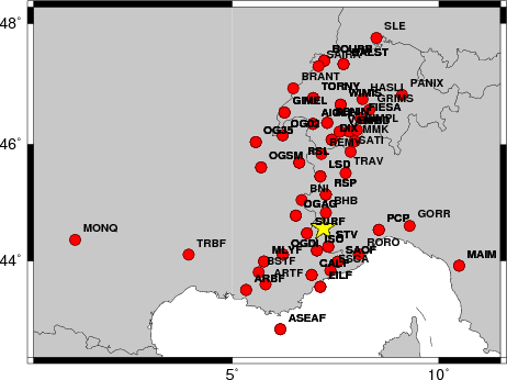
The focal mechanism was determined using broadband seismic waveforms. The location of the event and the and stations used for the waveform inversion are shown in the next figure.

Location of broadband stations used for waveform inversion

The program wvfgrd96 was used with good traces observed at short distance to determine the focal mechanism, depth and seismic moment. This technique requires a high quality signal and well determined velocity model for the Green functions. To the extent that these are the quality data, this type of mechanism should be preferred over the radiation pattern technique which requires the separate step of defining the pressure and tension quadrants and the correct strike.

The observed and predicted traces are filtered using the following gsac commands:

hp c 0.02 n 3
lp c 0.10 n 3

The results of this grid search from 0.5 to 19 km depth are as follow:

           DEPTH  STK   DIP  RAKE   MW    FIT
WVFGRD96    1.0   315    30   -85   3.64 0.3254
WVFGRD96    2.0   200    10   -25   3.78 0.3455
WVFGRD96    3.0   200    10   -30   3.76 0.4641
WVFGRD96    4.0   185    10   -45   3.74 0.5263
WVFGRD96    5.0   185    15   -50   3.86 0.5737
WVFGRD96    6.0   175    15   -60   3.86 0.6112
WVFGRD96    7.0   180    20   -55   3.87 0.6287
WVFGRD96    8.0   175    20   -65   3.84 0.6290
WVFGRD96    9.0   180    20   -60   3.84 0.6220
WVFGRD96   10.0   185    20   -55   3.85 0.6103
WVFGRD96   11.0   190    20   -45   3.84 0.5953
WVFGRD96   12.0   190    20   -45   3.85 0.5785
WVFGRD96   13.0   195    20   -40   3.85 0.5607
WVFGRD96   14.0   200    20   -35   3.86 0.5439
WVFGRD96   15.0   205    20   -30   3.91 0.5298
WVFGRD96   16.0   205    20   -30   3.92 0.5116
WVFGRD96   17.0   200    15   -35   3.92 0.4940
WVFGRD96   18.0   205    15   -30   3.93 0.4774
WVFGRD96   19.0   205    15   -30   3.94 0.4606
WVFGRD96   20.0   215    15   -20   3.95 0.4430
WVFGRD96   21.0   215    15   -20   3.96 0.4263
WVFGRD96   22.0   225    15   -10   3.97 0.4089
WVFGRD96   23.0   230    15    -5   3.98 0.3933
WVFGRD96   24.0   235    15     0   3.98 0.3785
WVFGRD96   25.0   245    15    10   3.99 0.3646
WVFGRD96   26.0   265    15    30   3.99 0.3532
WVFGRD96   27.0   280    25    45   3.99 0.3450
WVFGRD96   28.0   285    20    50   3.99 0.3398
WVFGRD96   29.0   290    20    55   4.00 0.3339

The best solution is

WVFGRD96    8.0   175    20   -65   3.84 0.6290

The mechanism correspond to the best fit is

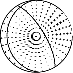
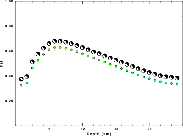
Figure 1. Waveform inversion focal mechanism

The best fit as a function of depth is given in the following figure:

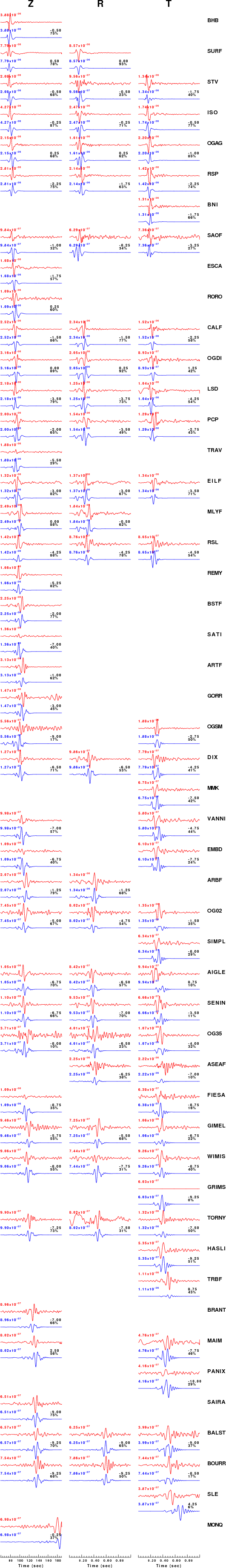
Figure 2. Depth sensitivity for waveform mechanism

The comparison of the observed and predicted waveforms is given in the next figure. The red traces are the observed and the blue are the predicted. Each observed-predicted component is plotted to the same scale and peak amplitudes are indicated by the numbers to the left of each trace. A pair of numbers is given in black at the right of each predicted traces. The upper number it the time shift required for maximum correlation between the observed and predicted traces. This time shift is required because the synthetics are not computed at exactly the same distance as the observed and because the velocity model used in the predictions may not be perfect. A positive time shift indicates that the prediction is too fast and should be delayed to match the observed trace (shift to the right in this figure). A negative value indicates that the prediction is too slow. The lower number gives the percentage of variance reduction to characterize the individual goodness of fit (100% indicates a perfect fit).

The bandpass filter used in the processing and for the display was

hp c 0.02 n 3
lp c 0.10 n 3

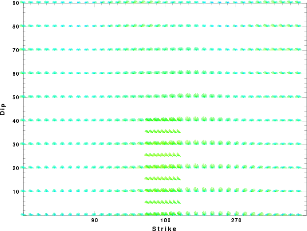
Figure 3. Waveform comparison for selected depth

Focal mechanism sensitivity at the preferred depth. The red color indicates a very good fit to thewavefroms. Each solution is plotted as a vector at a given value of strike and dip with the angle of the vector representing the rake angle, measured, with respect to the upward vertical (N) in the figure.

A check on the assumed source location is possible by looking at the time shifts between the observed and predicted traces. The time shifts for waveform matching arise for several reasons:

The origin time and epicentral distance are incorrect
The velocity model used for the inversion is incorrect
The velocity model used to define the P-arrival time is not the same as the velocity model used for the waveform inversion (assuming that the initial trace alignment is based on the P arrival time)

Assuming only a mislocation, the time shifts are fit to a functional form:

 Time_shift = A + B cos Azimuth + C Sin Azimuth

The time shifts for this inversion lead to the next figure:

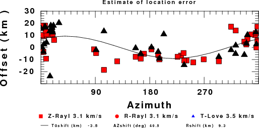
The derived shift in origin time and epicentral coordinates are given at the bottom of the figure.

Discussion

Velocity Model

The nnCIA used for the waveform synthetic seismograms and for the surface wave eigenfunctions and dispersion is as follows:

MODEL.01
C.It. A. Di Luzio et al Earth Plan Lettrs 280 (2009) 1-12 Fig 5. 7-8 MODEL/SURF3
ISOTROPIC
KGS
FLAT EARTH
1-D
CONSTANT VELOCITY
LINE08
LINE09
LINE10
LINE11
      H(KM)   VP(KM/S)   VS(KM/S) RHO(GM/CC)         QP         QS       ETAP       ETAS      FREFP      FREFS
     1.5000     3.7497     2.1436     2.2753  0.500E-02  0.100E-01   0.00       0.00       1.00       1.00    
     3.0000     4.9399     2.8210     2.4858  0.500E-02  0.100E-01   0.00       0.00       1.00       1.00    
     3.0000     6.0129     3.4336     2.7058  0.500E-02  0.100E-01   0.00       0.00       1.00       1.00    
     7.0000     5.5516     3.1475     2.6093  0.167E-02  0.333E-02   0.00       0.00       1.00       1.00    
    15.0000     5.8805     3.3583     2.6770  0.167E-02  0.333E-02   0.00       0.00       1.00       1.00    
     6.0000     7.1059     4.0081     3.0002  0.167E-02  0.333E-02   0.00       0.00       1.00       1.00    
     8.0000     7.1000     3.9864     3.0120  0.167E-02  0.333E-02   0.00       0.00       1.00       1.00    
     0.0000     7.9000     4.4036     3.2760  0.167E-02  0.333E-02   0.00       0.00       1.00       1.00

Quality Control

Here we tabulate the reasons for not using certain digital data sets

The following stations did not have a valid response files:

DATE=Wed Oct 3 08:20:06 CDT 2012

Last Changed 2012/10/03