Location
2012/01/25 08:06:36 44.854 10.538 33.2 4.9 Italy
Arrival Times (from USGS)
Arrival time list
Felt Map
USGS Felt map for this earthquake
USGS Felt reports page for
Focal Mechanism
 SLU Moment Tensor Solution
 ENS  2012/01/25 08:06:36:0  44.85   10.54  33.2 4.9 Italy

 Stations used:
   GU.MAIM GU.PCP GU.POPM GU.SC2M IV.ASQU IV.BOB IV.CAFI
   IV.CRE IV.CRMI IV.CSNT IV.FNVD IV.FROS IV.MABI IV.MAGA
   IV.MSSA IV.MTRZ IV.PARC IV.QLNO IV.ROVR IV.SALO IV.TEOL
   IV.VARE IV.ZCCA MN.TUE MN.VLC NI.CGRP

 Filtering commands used:
   hp c 0.02 n 3
   lp c 0.05 n 3

 Best Fitting Double Couple
  Mo = 2.07e+23 dyne-cm
  Mw = 4.81
  Z  = 26 km
  Plane   Strike  Dip  Rake
   NP1       82    80   -118
   NP2      335    30   -20
  Principal Axes:
   Axis    Value   Plunge  Azimuth
    T   2.07e+23     29     195
    N   0.00e+00     28      88
    P  -2.07e+23     47     323

 Moment Tensor: (dyne-cm)
    Component   Value
       Mxx     8.53e+22
       Mxy     8.58e+22
       Mxz    -1.67e+23
       Myy    -2.41e+22
       Myz     3.90e+22
       Mzz    -6.12e+22


                     ##############
                 -------------#########
              -------------------#########
             -----------------------#######
           --------------------------########
          ----------   ----------------#######
         ----------- P -----------------#######
        ------------   ------------------#######
        ----------------------------------######
       ------------------------------------######
       ------------------------------------#-----
       ------------------------------######------
       #------------------#################------
        ###################################-----
        ###################################-----
         ##################################----
          ################################----
           ############   ################---
             ########## T ###############--
              #########   ##############--
                 #####################-
                     ##############


 Global CMT Convention Moment Tensor:
      R          T          P
 -6.12e+22  -1.67e+23  -3.90e+22
 -1.67e+23   8.53e+22  -8.58e+22
 -3.90e+22  -8.58e+22  -2.41e+22


Details of the solution is found at

http://www.eas.slu.edu/eqc/eqc_mt/MECH.IT/20120125080636/index.html
|
Preferred Solution
The preferred solution from an analysis of the surface-wave spectral amplitude radiation pattern, waveform inversion and first motion observations is
      STK = 335
      DIP = 30
     RAKE = -20
       MW = 4.81
       HS = 26.0
The waveform inversion is preferred.
Moment Tensor Comparison
The following compares this source inversion to others
| SLU |
INGVTDMT |
 SLU Moment Tensor Solution
 ENS  2012/01/25 08:06:36:0  44.85   10.54  33.2 4.9 Italy

 Stations used:
   GU.MAIM GU.PCP GU.POPM GU.SC2M IV.ASQU IV.BOB IV.CAFI
   IV.CRE IV.CRMI IV.CSNT IV.FNVD IV.FROS IV.MABI IV.MAGA
   IV.MSSA IV.MTRZ IV.PARC IV.QLNO IV.ROVR IV.SALO IV.TEOL
   IV.VARE IV.ZCCA MN.TUE MN.VLC NI.CGRP

 Filtering commands used:
   hp c 0.02 n 3
   lp c 0.05 n 3

 Best Fitting Double Couple
  Mo = 2.07e+23 dyne-cm
  Mw = 4.81
  Z  = 26 km
  Plane   Strike  Dip  Rake
   NP1       82    80   -118
   NP2      335    30   -20
  Principal Axes:
   Axis    Value   Plunge  Azimuth
    T   2.07e+23     29     195
    N   0.00e+00     28      88
    P  -2.07e+23     47     323

 Moment Tensor: (dyne-cm)
    Component   Value
       Mxx     8.53e+22
       Mxy     8.58e+22
       Mxz    -1.67e+23
       Myy    -2.41e+22
       Myz     3.90e+22
       Mzz    -6.12e+22


                     ##############
                 -------------#########
              -------------------#########
             -----------------------#######
           --------------------------########
          ----------   ----------------#######
         ----------- P -----------------#######
        ------------   ------------------#######
        ----------------------------------######
       ------------------------------------######
       ------------------------------------#-----
       ------------------------------######------
       #------------------#################------
        ###################################-----
        ###################################-----
         ##################################----
          ################################----
           ############   ################---
             ########## T ###############--
              #########   ##############--
                 #####################-
                     ##############


 Global CMT Convention Moment Tensor:
      R          T          P
 -6.12e+22  -1.67e+23  -3.90e+22
 -1.67e+23   8.53e+22  -8.58e+22
 -3.90e+22  -8.58e+22  -2.41e+22


Details of the solution is found at

http://www.eas.slu.edu/eqc/eqc_mt/MECH.IT/20120125080636/index.html
|
|
Waveform Inversion
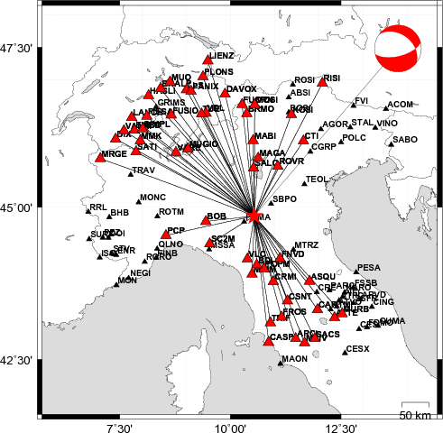
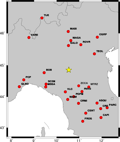
The focal mechanism was determined using broadband seismic waveforms. The location of the event and the
and stations used for the waveform inversion are shown in the next figure.
|
|
Location of broadband stations used for waveform inversion
|
The program wvfgrd96 was used with good traces observed at short distance to determine the focal mechanism, depth and seismic moment. This technique requires a high quality signal and well determined velocity model for the Green functions. To the extent that these are the quality data, this type of mechanism should be preferred over the radiation pattern technique which requires the separate step of defining the pressure and tension quadrants and the correct strike.
The observed and predicted traces are filtered using the following gsac commands:
hp c 0.02 n 3
lp c 0.05 n 3
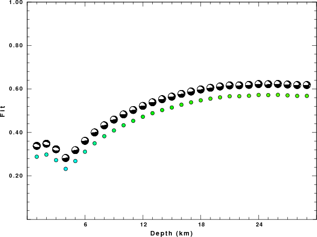
The results of this grid search from 0.5 to 19 km depth are as follow:
           DEPTH  STK   DIP  RAKE   MW    FIT
WVFGRD96    1.0    95    50  -100   4.51 0.2883
WVFGRD96    2.0   285    40   -85   4.57 0.2982
WVFGRD96    3.0   285    40   -85   4.61 0.2726
WVFGRD96    4.0   340    25   -10   4.61 0.2325
WVFGRD96    5.0   340    20   -10   4.71 0.2685
WVFGRD96    6.0   340    20   -10   4.71 0.3114
WVFGRD96    7.0   340    20   -10   4.71 0.3501
WVFGRD96    8.0   340    25   -10   4.67 0.3827
WVFGRD96    9.0   340    25   -10   4.67 0.4091
WVFGRD96   10.0   340    25   -15   4.68 0.4331
WVFGRD96   11.0   340    25   -15   4.68 0.4534
WVFGRD96   12.0   340    25   -15   4.69 0.4722
WVFGRD96   13.0   340    25   -15   4.69 0.4888
WVFGRD96   14.0   340    30   -15   4.70 0.5031
WVFGRD96   15.0   335    25   -20   4.74 0.5148
WVFGRD96   16.0   335    25   -20   4.75 0.5275
WVFGRD96   17.0   335    25   -20   4.75 0.5384
WVFGRD96   18.0   335    25   -20   4.76 0.5478
WVFGRD96   19.0   335    25   -20   4.77 0.5555
WVFGRD96   20.0   335    25   -20   4.77 0.5615
WVFGRD96   21.0   335    30   -20   4.78 0.5664
WVFGRD96   22.0   330    30   -25   4.79 0.5668
WVFGRD96   23.0   330    30   -25   4.80 0.5688
WVFGRD96   24.0   335    30   -20   4.80 0.5726
WVFGRD96   25.0   335    30   -20   4.81 0.5721
WVFGRD96   26.0   335    30   -20   4.81 0.5730
WVFGRD96   27.0   335    30   -20   4.82 0.5706
WVFGRD96   28.0   340    35   -15   4.82 0.5682
WVFGRD96   29.0   340    35   -15   4.83 0.5682
The best solution is
WVFGRD96 26.0 335 30 -20 4.81 0.5730
The mechanism correspond to the best fit is
|
|
Figure 1. Waveform inversion focal mechanism
|
The best fit as a function of depth is given in the following figure:
|
|
Figure 2. Depth sensitivity for waveform mechanism
|
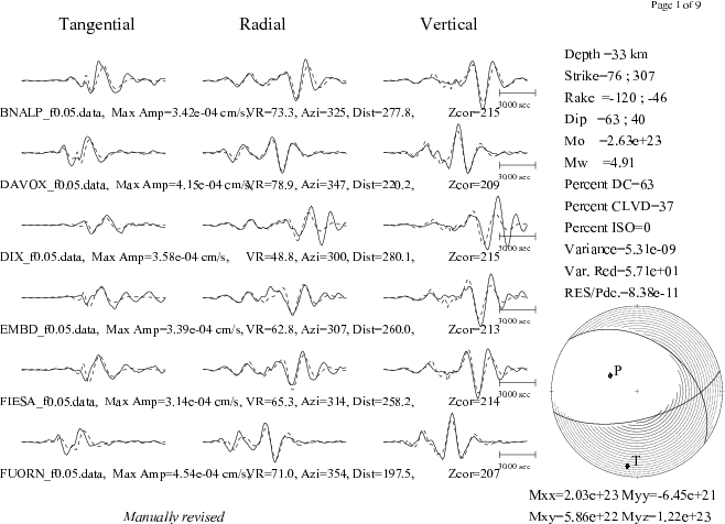
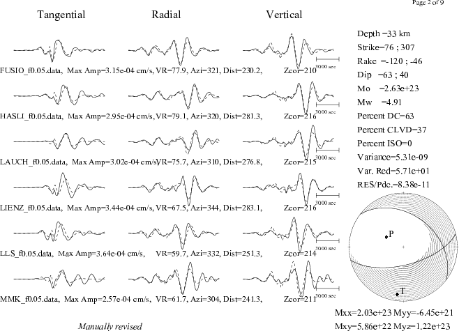
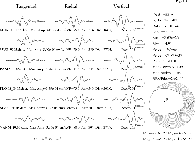
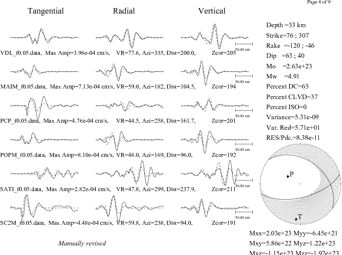
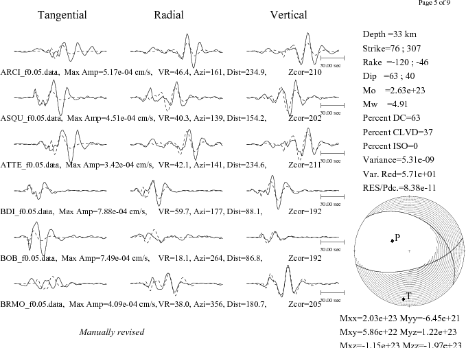
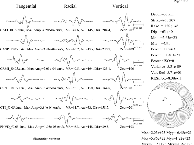
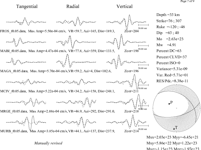
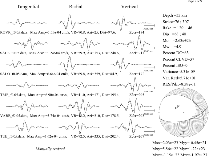
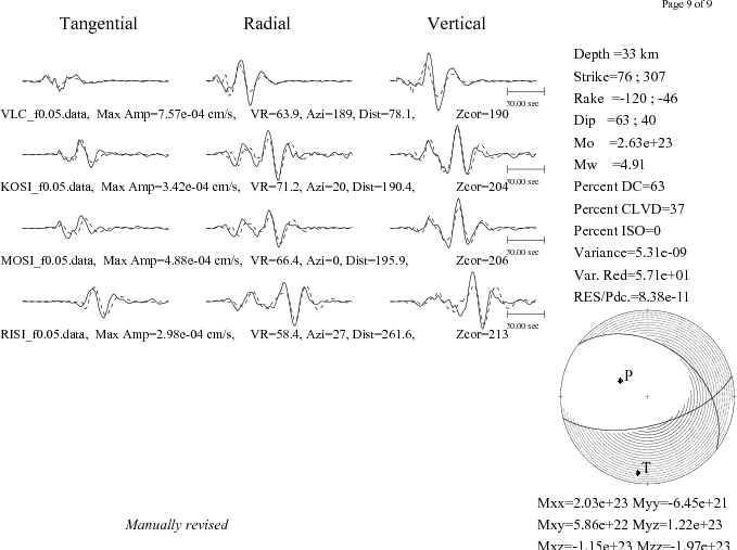
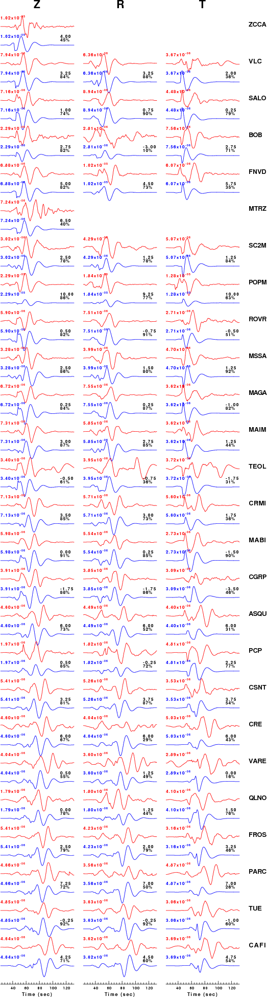
The comparison of the observed and predicted waveforms is given in the next figure. The red traces are the observed and the blue are the predicted.
Each observed-predicted component is plotted to the same scale and peak amplitudes are indicated by the numbers to the left of each trace. A pair of numbers is given in black at the right of each predicted traces. The upper number it the time shift required for maximum correlation between the observed and predicted traces. This time shift is required because the synthetics are not computed at exactly the same distance as the observed and because the velocity model used in the predictions may not be perfect.
A positive time shift indicates that the prediction is too fast and should be delayed to match the observed trace (shift to the right in this figure). A negative value indicates that the prediction is too slow. The lower number gives the percentage of variance reduction to characterize the individual goodness of fit (100% indicates a perfect fit).
The bandpass filter used in the processing and for the display was
hp c 0.02 n 3
lp c 0.05 n 3
|
|
Figure 3. Waveform comparison for selected depth
|
|
|
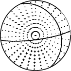
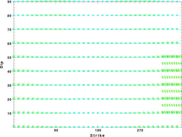
Focal mechanism sensitivity at the preferred depth. The red color indicates a very good fit to thewavefroms.
Each solution is plotted as a vector at a given value of strike and dip with the angle of the vector representing the rake angle, measured, with respect to the upward vertical (N) in the figure.
|
A check on the assumed source location is possible by looking at the time shifts between the observed and predicted traces. The time shifts for waveform matching arise for several reasons:
- The origin time and epicentral distance are incorrect
- The velocity model used for the inversion is incorrect
- The velocity model used to define the P-arrival time is not the
same as the velocity model used for the waveform inversion
(assuming that the initial trace alignment is based on the
P arrival time)
Assuming only a mislocation, the time shifts are fit to a functional form:
Time_shift = A + B cos Azimuth + C Sin Azimuth
The time shifts for this inversion lead to the next figure:
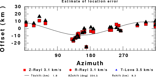
The derived shift in origin time and epicentral coordinates are given at the bottom of the figure.
Discussion
Velocity Model
The nnCIA used for the waveform synthetic seismograms and for the surface wave eigenfunctions and dispersion is as follows:
MODEL.01
C.It. A. Di Luzio et al Earth Plan Lettrs 280 (2009) 1-12 Fig 5. 7-8 MODEL/SURF3
ISOTROPIC
KGS
FLAT EARTH
1-D
CONSTANT VELOCITY
LINE08
LINE09
LINE10
LINE11
      H(KM)   VP(KM/S)   VS(KM/S) RHO(GM/CC)         QP         QS       ETAP       ETAS      FREFP      FREFS
     1.5000     3.7497     2.1436     2.2753  0.500E-02  0.100E-01   0.00       0.00       1.00       1.00
     3.0000     4.9399     2.8210     2.4858  0.500E-02  0.100E-01   0.00       0.00       1.00       1.00
     3.0000     6.0129     3.4336     2.7058  0.500E-02  0.100E-01   0.00       0.00       1.00       1.00
     7.0000     5.5516     3.1475     2.6093  0.167E-02  0.333E-02   0.00       0.00       1.00       1.00
    15.0000     5.8805     3.3583     2.6770  0.167E-02  0.333E-02   0.00       0.00       1.00       1.00
     6.0000     7.1059     4.0081     3.0002  0.167E-02  0.333E-02   0.00       0.00       1.00       1.00
     8.0000     7.1000     3.9864     3.0120  0.167E-02  0.333E-02   0.00       0.00       1.00       1.00
     0.0000     7.9000     4.4036     3.2760  0.167E-02  0.333E-02   0.00       0.00       1.00       1.00
Quality Control
Here we tabulate the reasons for not using certain digital data sets
The following stations did not have a valid response files:
DATE=Fri Feb 17 07:46:16 CST 2012
Last Changed 2012/01/25