Location

2011/10/30 14:40:32 42.274 13.323 8.2 3.6 Italy

Arrival Times (from USGS)

Felt Map

Focal Mechanism

SLU Moment Tensor Solution ENS 2011/10/30 14:40:32:0 42.27 13.32 8.2 3.6 Italy Stations used: IV.CAFR IV.CERT IV.CESI IV.CESX IV.CING IV.FAGN IV.FDMO IV.FIAM IV.FRES IV.GIUL IV.GUMA IV.LATE IV.MA9 IV.MGAB IV.MIDA IV.MODR IV.MTCE IV.MURB IV.NRCA IV.POFI IV.PTQR IV.RDP IV.RMP IV.RNI2 IV.ROM9 IV.SACS IV.SAMA IV.SNTG IV.SSFR IV.TERO IV.TOLF IV.TRTR IV.VVLD MN.AQU Filtering commands used: hp c 0.02 n 3 lp c 0.10 n 3 Best Fitting Double Couple Mo = 2.75e+21 dyne-cm Mw = 3.56 Z = 1 km Plane Strike Dip Rake NP1 138 50 -94 NP2 325 40 -85 Principal Axes: Axis Value Plunge Azimuth T 2.75e+21 5 231 N 0.00e+00 3 141 P -2.75e+21 84 19 Moment Tensor: (dyne-cm) Component Value Mxx 1.03e+21 Mxy 1.32e+21 Mxz -4.24e+20 Myy 1.67e+21 Myz -2.85e+20 Mzz -2.70e+21 ############## ###################### --------------############## #-----------------############ ###--------------------########### ###-----------------------########## #####-----------------------########## ######-------------------------######### ######--------------------------######## ########------------ -----------######## #########----------- P -----------######## ##########---------- ------------####### ###########------------------------####### ###########------------------------##### ############-----------------------##### #############---------------------#### # ##########------------------#### T #############---------------### ################-----------## #######################----- ###################### ############## Global CMT Convention Moment Tensor: R T P -2.70e+21 -4.24e+20 2.85e+20 -4.24e+20 1.03e+21 -1.32e+21 2.85e+20 -1.32e+21 1.67e+21 Details of the solution is found at http://www.eas.slu.edu/eqc/eqc_mt/MECH.IT/20111030144032/index.html

Preferred Solution

The preferred solution from an analysis of the surface-wave spectral amplitude radiation pattern, waveform inversion and first motion observations is

      STK = 325
      DIP = 40
     RAKE = -85
       MW = 3.56
       HS = 1.0

The waveform inversion is preferred.

Moment Tensor Comparison

The following compares this source inversion to others

SLU

SLU Moment Tensor Solution ENS 2011/10/30 14:40:32:0 42.27 13.32 8.2 3.6 Italy Stations used: IV.CAFR IV.CERT IV.CESI IV.CESX IV.CING IV.FAGN IV.FDMO IV.FIAM IV.FRES IV.GIUL IV.GUMA IV.LATE IV.MA9 IV.MGAB IV.MIDA IV.MODR IV.MTCE IV.MURB IV.NRCA IV.POFI IV.PTQR IV.RDP IV.RMP IV.RNI2 IV.ROM9 IV.SACS IV.SAMA IV.SNTG IV.SSFR IV.TERO IV.TOLF IV.TRTR IV.VVLD MN.AQU Filtering commands used: hp c 0.02 n 3 lp c 0.10 n 3 Best Fitting Double Couple Mo = 2.75e+21 dyne-cm Mw = 3.56 Z = 1 km Plane Strike Dip Rake NP1 138 50 -94 NP2 325 40 -85 Principal Axes: Axis Value Plunge Azimuth T 2.75e+21 5 231 N 0.00e+00 3 141 P -2.75e+21 84 19 Moment Tensor: (dyne-cm) Component Value Mxx 1.03e+21 Mxy 1.32e+21 Mxz -4.24e+20 Myy 1.67e+21 Myz -2.85e+20 Mzz -2.70e+21 ############## ###################### --------------############## #-----------------############ ###--------------------########### ###-----------------------########## #####-----------------------########## ######-------------------------######### ######--------------------------######## ########------------ -----------######## #########----------- P -----------######## ##########---------- ------------####### ###########------------------------####### ###########------------------------##### ############-----------------------##### #############---------------------#### # ##########------------------#### T #############---------------### ################-----------## #######################----- ###################### ############## Global CMT Convention Moment Tensor: R T P -2.70e+21 -4.24e+20 2.85e+20 -4.24e+20 1.03e+21 -1.32e+21 2.85e+20 -1.32e+21 1.67e+21 Details of the solution is found at http://www.eas.slu.edu/eqc/eqc_mt/MECH.IT/20111030144032/index.html

Waveform Inversion

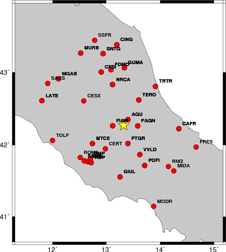
The focal mechanism was determined using broadband seismic waveforms. The location of the event and the and stations used for the waveform inversion are shown in the next figure.

Location of broadband stations used for waveform inversion

The program wvfgrd96 was used with good traces observed at short distance to determine the focal mechanism, depth and seismic moment. This technique requires a high quality signal and well determined velocity model for the Green functions. To the extent that these are the quality data, this type of mechanism should be preferred over the radiation pattern technique which requires the separate step of defining the pressure and tension quadrants and the correct strike.

The observed and predicted traces are filtered using the following gsac commands:

hp c 0.02 n 3
lp c 0.10 n 3

The results of this grid search from 0.5 to 19 km depth are as follow:

           DEPTH  STK   DIP  RAKE   MW    FIT
WVFGRD96    1.0   325    40   -85   3.56 0.5252
WVFGRD96    2.0   330    35   -75   3.61 0.4894
WVFGRD96    3.0   335    20   -70   3.61 0.4274
WVFGRD96    4.0   335    20   -70   3.59 0.4413
WVFGRD96    5.0   330    20   -75   3.69 0.4624
WVFGRD96    6.0   135    70   -95   3.69 0.4615
WVFGRD96    7.0   140    70   -90   3.70 0.4512
WVFGRD96    8.0   140    75   -75   3.64 0.4331
WVFGRD96    9.0   140    75   -75   3.64 0.4187
WVFGRD96   10.0    10    65    40   3.68 0.4098
WVFGRD96   11.0   315    70    75   3.66 0.4026
WVFGRD96   12.0   315    65    80   3.68 0.4038
WVFGRD96   13.0   320    60    80   3.70 0.4038
WVFGRD96   14.0   320    60    85   3.71 0.4029
WVFGRD96   15.0   320    60    85   3.75 0.3955
WVFGRD96   16.0   320    60    85   3.76 0.3895
WVFGRD96   17.0   320    60    85   3.77 0.3800
WVFGRD96   18.0   315    55    80   3.78 0.3713
WVFGRD96   19.0   315    55    80   3.79 0.3600
WVFGRD96   20.0   315    55    80   3.80 0.3470
WVFGRD96   21.0   310    55    75   3.80 0.3329
WVFGRD96   22.0   310    55    75   3.81 0.3188
WVFGRD96   23.0   315    50    80   3.81 0.3044
WVFGRD96   24.0   150    40   100   3.81 0.2905
WVFGRD96   25.0   155    50   110   3.82 0.2785
WVFGRD96   26.0   305    45    70   3.82 0.2709
WVFGRD96   27.0   300    45    65   3.83 0.2639
WVFGRD96   28.0   150    55   -70   3.84 0.2532
WVFGRD96   29.0   145    50   -80   3.85 0.2479

The best solution is

WVFGRD96    1.0   325    40   -85   3.56 0.5252

The mechanism correspond to the best fit is

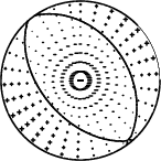
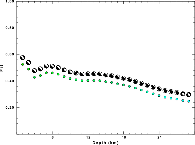
Figure 1. Waveform inversion focal mechanism

The best fit as a function of depth is given in the following figure:

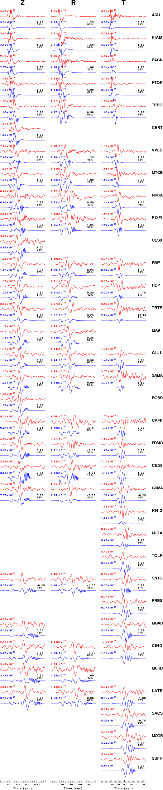
Figure 2. Depth sensitivity for waveform mechanism

The comparison of the observed and predicted waveforms is given in the next figure. The red traces are the observed and the blue are the predicted. Each observed-predicted component is plotted to the same scale and peak amplitudes are indicated by the numbers to the left of each trace. A pair of numbers is given in black at the right of each predicted traces. The upper number it the time shift required for maximum correlation between the observed and predicted traces. This time shift is required because the synthetics are not computed at exactly the same distance as the observed and because the velocity model used in the predictions may not be perfect. A positive time shift indicates that the prediction is too fast and should be delayed to match the observed trace (shift to the right in this figure). A negative value indicates that the prediction is too slow. The lower number gives the percentage of variance reduction to characterize the individual goodness of fit (100% indicates a perfect fit).

The bandpass filter used in the processing and for the display was

hp c 0.02 n 3
lp c 0.10 n 3

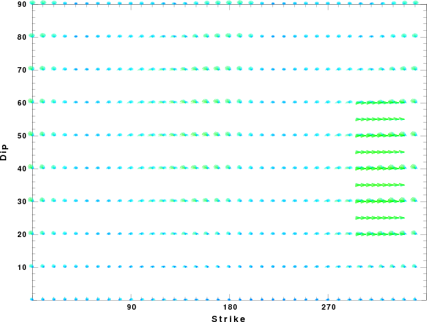
Figure 3. Waveform comparison for selected depth

Focal mechanism sensitivity at the preferred depth. The red color indicates a very good fit to thewavefroms. Each solution is plotted as a vector at a given value of strike and dip with the angle of the vector representing the rake angle, measured, with respect to the upward vertical (N) in the figure.

A check on the assumed source location is possible by looking at the time shifts between the observed and predicted traces. The time shifts for waveform matching arise for several reasons:

The origin time and epicentral distance are incorrect
The velocity model used for the inversion is incorrect
The velocity model used to define the P-arrival time is not the same as the velocity model used for the waveform inversion (assuming that the initial trace alignment is based on the P arrival time)

Assuming only a mislocation, the time shifts are fit to a functional form:

 Time_shift = A + B cos Azimuth + C Sin Azimuth

The time shifts for this inversion lead to the next figure:

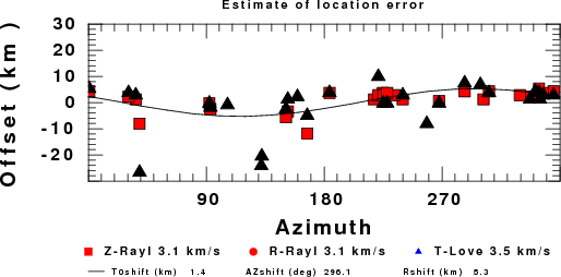
The derived shift in origin time and epicentral coordinates are given at the bottom of the figure.

Discussion

Velocity Model

The nnCIA used for the waveform synthetic seismograms and for the surface wave eigenfunctions and dispersion is as follows:

MODEL.01
C.It. A. Di Luzio et al Earth Plan Lettrs 280 (2009) 1-12 Fig 5. 7-8 MODEL/SURF3
ISOTROPIC
KGS
FLAT EARTH
1-D
CONSTANT VELOCITY
LINE08
LINE09
LINE10
LINE11
      H(KM)   VP(KM/S)   VS(KM/S) RHO(GM/CC)         QP         QS       ETAP       ETAS      FREFP      FREFS
     1.5000     3.7497     2.1436     2.2753  0.500E-02  0.100E-01   0.00       0.00       1.00       1.00    
     3.0000     4.9399     2.8210     2.4858  0.500E-02  0.100E-01   0.00       0.00       1.00       1.00    
     3.0000     6.0129     3.4336     2.7058  0.500E-02  0.100E-01   0.00       0.00       1.00       1.00    
     7.0000     5.5516     3.1475     2.6093  0.167E-02  0.333E-02   0.00       0.00       1.00       1.00    
    15.0000     5.8805     3.3583     2.6770  0.167E-02  0.333E-02   0.00       0.00       1.00       1.00    
     6.0000     7.1059     4.0081     3.0002  0.167E-02  0.333E-02   0.00       0.00       1.00       1.00    
     8.0000     7.1000     3.9864     3.0120  0.167E-02  0.333E-02   0.00       0.00       1.00       1.00    
     0.0000     7.9000     4.4036     3.2760  0.167E-02  0.333E-02   0.00       0.00       1.00       1.00

Quality Control

Here we tabulate the reasons for not using certain digital data sets

The following stations did not have a valid response files:

DATE=Wed Nov 2 19:32:22 CDT 2011

Last Changed 2011/10/30