2011/09/08 20:36:42 44.625 10.239 19.8 3.1 Italy
USGS Felt map for this earthquake
 SLU Moment Tensor Solution
 ENS  2011/09/08 20:36:42:0  44.62   10.24  19.8 3.1 Italy

 Stations used:
   GU.SC2M IV.ASQU IV.BDI IV.CRE IV.FNVD IV.FROS IV.MSSA
   IV.PARC MN.VLC

 Filtering commands used:
   hp c 0.02 n 3
   lp c 0.10 n 3

 Best Fitting Double Couple
  Mo = 1.48e+21 dyne-cm
  Mw = 3.38
  Z  = 20 km
  Plane   Strike  Dip  Rake
   NP1      105    80    91
   NP2      280    10    85
  Principal Axes:
   Axis    Value   Plunge  Azimuth
    T   1.48e+21     55      16
    N   0.00e+00      1     285
    P  -1.48e+21     35     194

 Moment Tensor: (dyne-cm)
    Component   Value
       Mxx    -4.81e+20
       Mxy    -1.07e+20
       Mxz     1.34e+21
       Myy    -2.29e+19
       Myz     3.65e+20
       Mzz     5.04e+20


                     --------------
                 ---###############----
              ---######################---
             -###########################--
           -###############################--
          -##################   #############-
         #################### T ##############-
        -####################   ###############-
        -######################################-
       ------###################################-
       ----------###############################-
       ---------------###########################
       ----------------------####################
        -----------------------------###########
        ----------------------------------------
         --------------------------------------
          ------------------------------------
           ------------   -------------------
             ---------- P -----------------
              ---------   ----------------
                 ----------------------
                     --------------


 Global CMT Convention Moment Tensor:
      R          T          P
  5.04e+20   1.34e+21  -3.65e+20
  1.34e+21  -4.81e+20   1.07e+20
 -3.65e+20   1.07e+20  -2.29e+19


Details of the solution is found at

http://www.eas.slu.edu/eqc/eqc_mt/MECH.IT/20110908203642/index.html
|
      STK = 280
      DIP = 10
     RAKE = 85
       MW = 3.38
       HS = 20.0
The waveform inversion is preferred.
The following compares this source inversion to others
 SLU Moment Tensor Solution
 ENS  2011/09/08 20:36:42:0  44.62   10.24  19.8 3.1 Italy

 Stations used:
   GU.SC2M IV.ASQU IV.BDI IV.CRE IV.FNVD IV.FROS IV.MSSA
   IV.PARC MN.VLC

 Filtering commands used:
   hp c 0.02 n 3
   lp c 0.10 n 3

 Best Fitting Double Couple
  Mo = 1.48e+21 dyne-cm
  Mw = 3.38
  Z  = 20 km
  Plane   Strike  Dip  Rake
   NP1      105    80    91
   NP2      280    10    85
  Principal Axes:
   Axis    Value   Plunge  Azimuth
    T   1.48e+21     55      16
    N   0.00e+00      1     285
    P  -1.48e+21     35     194

 Moment Tensor: (dyne-cm)
    Component   Value
       Mxx    -4.81e+20
       Mxy    -1.07e+20
       Mxz     1.34e+21
       Myy    -2.29e+19
       Myz     3.65e+20
       Mzz     5.04e+20


                     --------------
                 ---###############----
              ---######################---
             -###########################--
           -###############################--
          -##################   #############-
         #################### T ##############-
        -####################   ###############-
        -######################################-
       ------###################################-
       ----------###############################-
       ---------------###########################
       ----------------------####################
        -----------------------------###########
        ----------------------------------------
         --------------------------------------
          ------------------------------------
           ------------   -------------------
             ---------- P -----------------
              ---------   ----------------
                 ----------------------
                     --------------


 Global CMT Convention Moment Tensor:
      R          T          P
  5.04e+20   1.34e+21  -3.65e+20
  1.34e+21  -4.81e+20   1.07e+20
 -3.65e+20   1.07e+20  -2.29e+19


Details of the solution is found at

http://www.eas.slu.edu/eqc/eqc_mt/MECH.IT/20110908203642/index.html
|
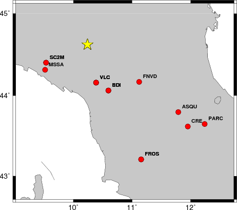
The focal mechanism was determined using broadband seismic waveforms. The location of the event and the and stations used for the waveform inversion are shown in the next figure.
|
|
|
|
The program wvfgrd96 was used with good traces observed at short distance to determine the focal mechanism, depth and seismic moment. This technique requires a high quality signal and well determined velocity model for the Green functions. To the extent that these are the quality data, this type of mechanism should be preferred over the radiation pattern technique which requires the separate step of defining the pressure and tension quadrants and the correct strike.
The observed and predicted traces are filtered using the following gsac commands:
hp c 0.02 n 3
lp c 0.10 n 3
The results of this grid search from 0.5 to 19 km depth are as follow:
           DEPTH  STK   DIP  RAKE   MW    FIT
WVFGRD96    1.0    80    40    85   2.99 0.2629
WVFGRD96    2.0   255    45    95   3.09 0.2918
WVFGRD96    3.0   205    90     0   3.18 0.2972
WVFGRD96    4.0   295    85     5   3.23 0.2809
WVFGRD96    5.0   300    80    10   3.28 0.2616
WVFGRD96    6.0   125    55    15   3.16 0.2312
WVFGRD96    7.0   130    45    15   3.13 0.2474
WVFGRD96    8.0   175    15   -15   3.07 0.2750
WVFGRD96    9.0   185    15    -5   3.10 0.3071
WVFGRD96   10.0   250     5    60   3.13 0.3397
WVFGRD96   11.0   260     5    70   3.15 0.3721
WVFGRD96   12.0   255    10    60   3.19 0.4029
WVFGRD96   13.0   270    10    75   3.21 0.4320
WVFGRD96   14.0   290    10    95   3.23 0.4586
WVFGRD96   15.0   280    10    85   3.29 0.4825
WVFGRD96   16.0   275    10    80   3.32 0.5066
WVFGRD96   17.0   275    10    80   3.34 0.5259
WVFGRD96   18.0   280    10    85   3.35 0.5399
WVFGRD96   19.0   280    10    85   3.37 0.5481
WVFGRD96   20.0   280    10    85   3.38 0.5504
WVFGRD96   21.0   280    10    85   3.39 0.5468
WVFGRD96   22.0   265    15    70   3.40 0.5399
WVFGRD96   23.0   260    15    65   3.41 0.5284
WVFGRD96   24.0   260    15    70   3.41 0.5134
WVFGRD96   25.0   240    20    50   3.42 0.4952
WVFGRD96   26.0   260    20    70   3.41 0.4773
WVFGRD96   27.0   155     5   -40   3.41 0.4600
WVFGRD96   28.0   135     5   -60   3.41 0.4482
WVFGRD96   29.0   145     5   -50   3.40 0.4345
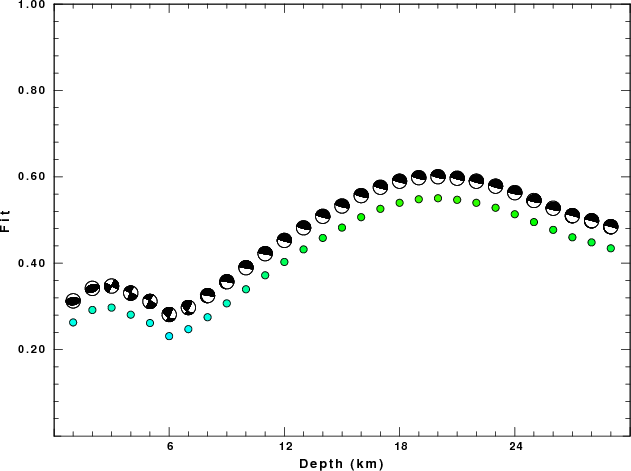
The best solution is
WVFGRD96 20.0 280 10 85 3.38 0.5504
The mechanism correspond to the best fit is
|
|
|
The best fit as a function of depth is given in the following figure:
|
|
|
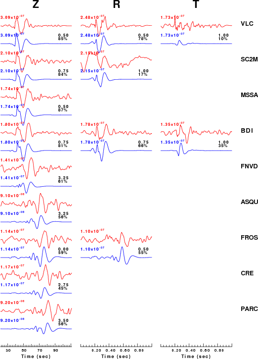
The comparison of the observed and predicted waveforms is given in the next figure. The red traces are the observed and the blue are the predicted. Each observed-predicted component is plotted to the same scale and peak amplitudes are indicated by the numbers to the left of each trace. A pair of numbers is given in black at the right of each predicted traces. The upper number it the time shift required for maximum correlation between the observed and predicted traces. This time shift is required because the synthetics are not computed at exactly the same distance as the observed and because the velocity model used in the predictions may not be perfect. A positive time shift indicates that the prediction is too fast and should be delayed to match the observed trace (shift to the right in this figure). A negative value indicates that the prediction is too slow. The lower number gives the percentage of variance reduction to characterize the individual goodness of fit (100% indicates a perfect fit).
The bandpass filter used in the processing and for the display was
hp c 0.02 n 3
lp c 0.10 n 3
|
|
|
|
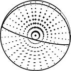
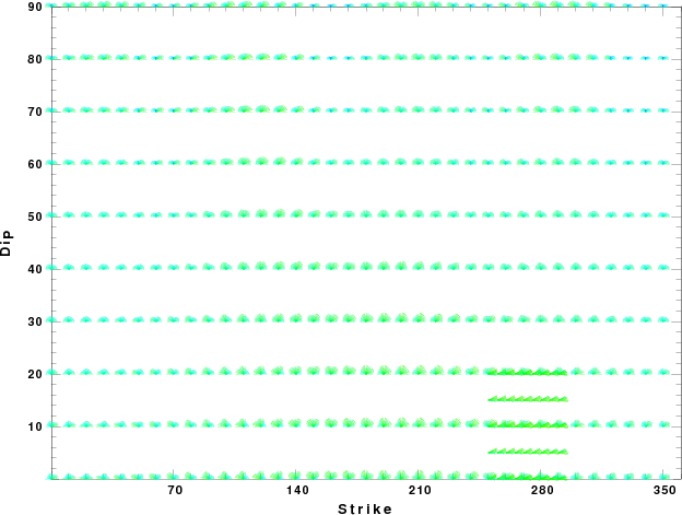
| Focal mechanism sensitivity at the preferred depth. The red color indicates a very good fit to thewavefroms. Each solution is plotted as a vector at a given value of strike and dip with the angle of the vector representing the rake angle, measured, with respect to the upward vertical (N) in the figure. |
A check on the assumed source location is possible by looking at the time shifts between the observed and predicted traces. The time shifts for waveform matching arise for several reasons:
Time_shift = A + B cos Azimuth + C Sin Azimuth
The time shifts for this inversion lead to the next figure:
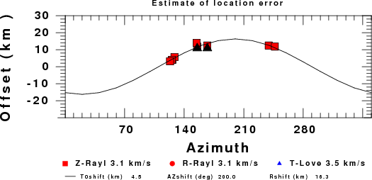
The derived shift in origin time and epicentral coordinates are given at the bottom of the figure.
The nnCIA used for the waveform synthetic seismograms and for the surface wave eigenfunctions and dispersion is as follows:
MODEL.01
C.It. A. Di Luzio et al Earth Plan Lettrs 280 (2009) 1-12 Fig 5. 7-8 MODEL/SURF3
ISOTROPIC
KGS
FLAT EARTH
1-D
CONSTANT VELOCITY
LINE08
LINE09
LINE10
LINE11
      H(KM)   VP(KM/S)   VS(KM/S) RHO(GM/CC)         QP         QS       ETAP       ETAS      FREFP      FREFS
     1.5000     3.7497     2.1436     2.2753  0.500E-02  0.100E-01   0.00       0.00       1.00       1.00
     3.0000     4.9399     2.8210     2.4858  0.500E-02  0.100E-01   0.00       0.00       1.00       1.00
     3.0000     6.0129     3.4336     2.7058  0.500E-02  0.100E-01   0.00       0.00       1.00       1.00
     7.0000     5.5516     3.1475     2.6093  0.167E-02  0.333E-02   0.00       0.00       1.00       1.00
    15.0000     5.8805     3.3583     2.6770  0.167E-02  0.333E-02   0.00       0.00       1.00       1.00
     6.0000     7.1059     4.0081     3.0002  0.167E-02  0.333E-02   0.00       0.00       1.00       1.00
     8.0000     7.1000     3.9864     3.0120  0.167E-02  0.333E-02   0.00       0.00       1.00       1.00
     0.0000     7.9000     4.4036     3.2760  0.167E-02  0.333E-02   0.00       0.00       1.00       1.00
Here we tabulate the reasons for not using certain digital data sets
The following stations did not have a valid response files:
DATE=Fri Sep 9 07:58:58 CDT 2011