2010/09/05 07:07:23 44.107 12.170 30.0 3.7 Italy
USGS Felt map for this earthquake
 USGS/SLU Moment Tensor Solution
 ENS  2010/09/05 07:07:23:0  44.11   12.17  30.0 3.7 Italy

 Stations used:
   GU.MAIM GU.SC2M IV.ARVD IV.ASQU IV.ATFO IV.ATPC IV.ATVO
   IV.BDI IV.CASP IV.CESI IV.CING IV.CRE IV.CRMI IV.CSNT
   IV.FIAM IV.FNVD IV.FSSB IV.GUMA IV.LATE IV.LNSS IV.MCIV
   IV.MGAB IV.MNS IV.MSSA IV.MTCE IV.MURB IV.PARC IV.ROVR
   IV.RSM IV.SACS IV.SASS IV.SNTG IV.TOLF IV.ZCCA MN.VLC

 Filtering commands used:
   hp c 0.02 n 3
   lp c 0.10 n 3

 Best Fitting Double Couple
  Mo = 4.95e+21 dyne-cm
  Mw = 3.73
  Z  = 17 km
  Plane   Strike  Dip  Rake
   NP1      318    62   101
   NP2      115    30    70
  Principal Axes:
   Axis    Value   Plunge  Azimuth
    T   4.95e+21     71     252
    N   0.00e+00     10     132
    P  -4.95e+21     16      40

 Moment Tensor: (dyne-cm)
    Component   Value
       Mxx    -2.66e+21
       Mxy    -2.09e+21
       Mxz    -1.49e+21
       Myy    -1.37e+21
       Myz    -2.31e+21
       Mzz     4.03e+21


                     --------------
                 ----------------------
              ------------------------   -
             ########----------------- P --
           ##############-------------   ----
          #################-------------------
         #####################-----------------
        -#######################----------------
        -########################---------------
       --##########################--------------
       ---############   ###########-------------
       ---############ T #############-----------
       ----###########   ##############----------
        ----############################--------
        -----###########################--------
         ------##########################------
          -------#########################---#
           --------#######################-##
             ----------#################--#
              ----------------------------
                 ----------------------
                     --------------


 Global CMT Convention Moment Tensor:
      R          T          P
  4.03e+21  -1.49e+21   2.31e+21
 -1.49e+21  -2.66e+21   2.09e+21
  2.31e+21   2.09e+21  -1.37e+21


Details of the solution is found at

http://www.eas.slu.edu/eqc/eqc_mt/MECH.IT/20100905070723/index.html
|
      STK = 115
      DIP = 30
     RAKE = 70
       MW = 3.73
       HS = 17.0
The waveform inversion is preferred.
The following compares this source inversion to others
 USGS/SLU Moment Tensor Solution
 ENS  2010/09/05 07:07:23:0  44.11   12.17  30.0 3.7 Italy

 Stations used:
   GU.MAIM GU.SC2M IV.ARVD IV.ASQU IV.ATFO IV.ATPC IV.ATVO
   IV.BDI IV.CASP IV.CESI IV.CING IV.CRE IV.CRMI IV.CSNT
   IV.FIAM IV.FNVD IV.FSSB IV.GUMA IV.LATE IV.LNSS IV.MCIV
   IV.MGAB IV.MNS IV.MSSA IV.MTCE IV.MURB IV.PARC IV.ROVR
   IV.RSM IV.SACS IV.SASS IV.SNTG IV.TOLF IV.ZCCA MN.VLC

 Filtering commands used:
   hp c 0.02 n 3
   lp c 0.10 n 3

 Best Fitting Double Couple
  Mo = 4.95e+21 dyne-cm
  Mw = 3.73
  Z  = 17 km
  Plane   Strike  Dip  Rake
   NP1      318    62   101
   NP2      115    30    70
  Principal Axes:
   Axis    Value   Plunge  Azimuth
    T   4.95e+21     71     252
    N   0.00e+00     10     132
    P  -4.95e+21     16      40

 Moment Tensor: (dyne-cm)
    Component   Value
       Mxx    -2.66e+21
       Mxy    -2.09e+21
       Mxz    -1.49e+21
       Myy    -1.37e+21
       Myz    -2.31e+21
       Mzz     4.03e+21


                     --------------
                 ----------------------
              ------------------------   -
             ########----------------- P --
           ##############-------------   ----
          #################-------------------
         #####################-----------------
        -#######################----------------
        -########################---------------
       --##########################--------------
       ---############   ###########-------------
       ---############ T #############-----------
       ----###########   ##############----------
        ----############################--------
        -----###########################--------
         ------##########################------
          -------#########################---#
           --------#######################-##
             ----------#################--#
              ----------------------------
                 ----------------------
                     --------------


 Global CMT Convention Moment Tensor:
      R          T          P
  4.03e+21  -1.49e+21   2.31e+21
 -1.49e+21  -2.66e+21   2.09e+21
  2.31e+21   2.09e+21  -1.37e+21


Details of the solution is found at

http://www.eas.slu.edu/eqc/eqc_mt/MECH.IT/20100905070723/index.html
|
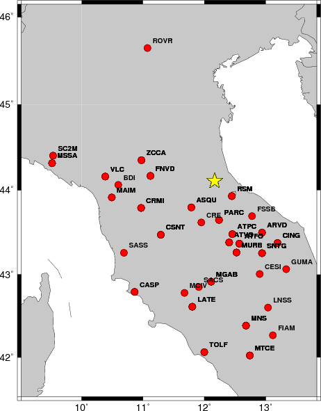
The focal mechanism was determined using broadband seismic waveforms. The location of the event and the and stations used for the waveform inversion are shown in the next figure.
|
|
|
|
The program wvfgrd96 was used with good traces observed at short distance to determine the focal mechanism, depth and seismic moment. This technique requires a high quality signal and well determined velocity model for the Green functions. To the extent that these are the quality data, this type of mechanism should be preferred over the radiation pattern technique which requires the separate step of defining the pressure and tension quadrants and the correct strike.
The observed and predicted traces are filtered using the following gsac commands:
hp c 0.02 n 3
lp c 0.10 n 3
The results of this grid search from 0.5 to 19 km depth are as follow:
           DEPTH  STK   DIP  RAKE   MW    FIT
WVFGRD96    1.0   325    45   -90   3.41 0.2506
WVFGRD96    2.0   145    40   -85   3.45 0.2120
WVFGRD96    3.0   350    20   -45   3.43 0.1784
WVFGRD96    4.0   120    80    80   3.40 0.2030
WVFGRD96    5.0   160   -10   -50   3.52 0.2375
WVFGRD96    6.0   305    10    90   3.55 0.2804
WVFGRD96    7.0   305    15    90   3.57 0.3218
WVFGRD96    8.0   125    70    90   3.55 0.3612
WVFGRD96    9.0   130    65    80   3.58 0.3916
WVFGRD96   10.0   115    30    75   3.60 0.4199
WVFGRD96   11.0   115    30    70   3.62 0.4443
WVFGRD96   12.0   115    30    70   3.63 0.4632
WVFGRD96   13.0   115    30    70   3.65 0.4779
WVFGRD96   14.0   115    35    70   3.66 0.4901
WVFGRD96   15.0   115    30    70   3.71 0.5004
WVFGRD96   16.0   115    30    70   3.72 0.5073
WVFGRD96   17.0   115    30    70   3.73 0.5105
WVFGRD96   18.0   115    30    70   3.74 0.5104
WVFGRD96   19.0   115    30    70   3.75 0.5069
WVFGRD96   20.0   115    30    70   3.76 0.4997
WVFGRD96   21.0   115    30    70   3.77 0.4890
WVFGRD96   22.0   115    30    70   3.78 0.4752
WVFGRD96   23.0   125    25    75   3.79 0.4591
WVFGRD96   24.0   120    25    70   3.80 0.4414
WVFGRD96   25.0   115    25    65   3.80 0.4199
WVFGRD96   26.0   110    25    60   3.80 0.3961
WVFGRD96   27.0   110    25    60   3.80 0.3741
WVFGRD96   28.0   105    25    55   3.80 0.3523
WVFGRD96   29.0   100    25    50   3.80 0.3324
The best solution is
WVFGRD96 17.0 115 30 70 3.73 0.5105
The mechanism correspond to the best fit is
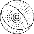
|
|
|
The best fit as a function of depth is given in the following figure:
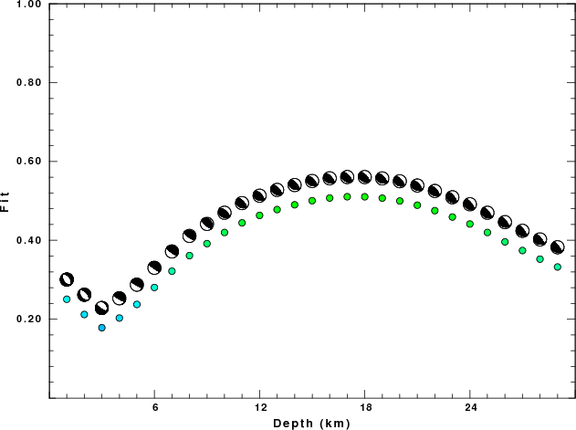
|
|
|
The comparison of the observed and predicted waveforms is given in the next figure. The red traces are the observed and the blue are the predicted. Each observed-predicted component is plotted to the same scale and peak amplitudes are indicated by the numbers to the left of each trace. The number in black at the rightr of each predicted traces it the time shift required for maximum correlation between the observed and predicted traces. This time shift is required because the synthetics are not computed at exactly the same distance as the observed and because the velocity model used in the predictions may not be perfect. A positive time shift indicates that the prediction is too fast and should be delayed to match the observed trace (shift to the right in this figure). A negative value indicates that the prediction is too slow. The bandpass filter used in the processing and for the display was
hp c 0.02 n 3
lp c 0.10 n 3
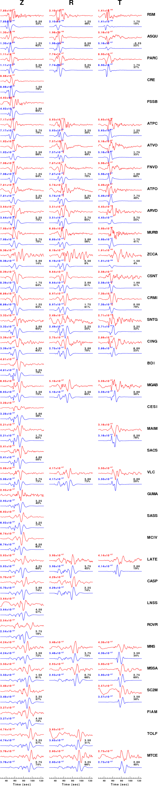
|
|
|
|
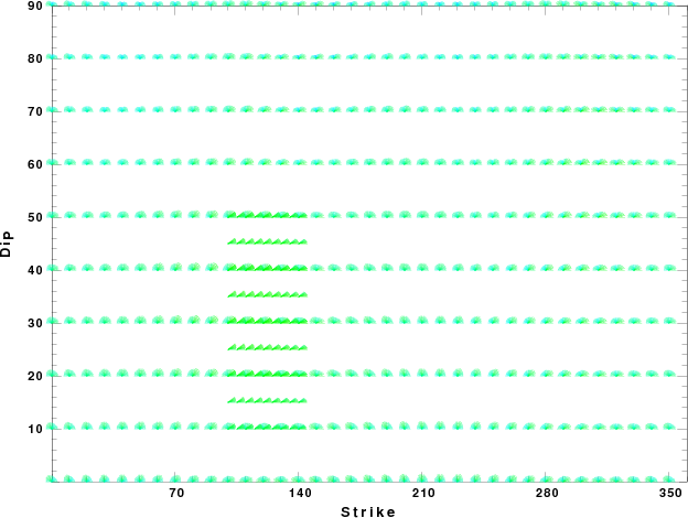
| Focal mechanism sensitivity at the preferred depth. The red color indicates a very good fit to thewavefroms. Each solution is plotted as a vector at a given value of strike and dip with the angle of the vector representing the rake angle, measured, with respect to the upward vertical (N) in the figure. |
The nnCIA used for the waveform synthetic seismograms and for the surface wave eigenfunctions and dispersion is as follows:
MODEL.01
C.It. A. Di Luzio et al Earth Plan Lettrs 280 (2009) 1-12 Fig 5. 7-8 MODEL/SURF3
ISOTROPIC
KGS
FLAT EARTH
1-D
CONSTANT VELOCITY
LINE08
LINE09
LINE10
LINE11
      H(KM)   VP(KM/S)   VS(KM/S) RHO(GM/CC)         QP         QS       ETAP       ETAS      FREFP      FREFS
     1.5000     3.7497     2.1436     2.2753  0.500E-02  0.100E-01   0.00       0.00       1.00       1.00
     3.0000     4.9399     2.8210     2.4858  0.500E-02  0.100E-01   0.00       0.00       1.00       1.00
     3.0000     6.0129     3.4336     2.7058  0.500E-02  0.100E-01   0.00       0.00       1.00       1.00
     7.0000     5.5516     3.1475     2.6093  0.167E-02  0.333E-02   0.00       0.00       1.00       1.00
    15.0000     5.8805     3.3583     2.6770  0.167E-02  0.333E-02   0.00       0.00       1.00       1.00
     6.0000     7.1059     4.0081     3.0002  0.167E-02  0.333E-02   0.00       0.00       1.00       1.00
     8.0000     7.1000     3.9864     3.0120  0.167E-02  0.333E-02   0.00       0.00       1.00       1.00
     0.0000     7.9000     4.4036     3.2760  0.167E-02  0.333E-02   0.00       0.00       1.00       1.00
Here we tabulate the reasons for not using certain digital data sets
The following stations did not have a valid response files:
DATE=Sun Sep 5 06:58:13 CDT 2010