Location
2010/08/28 07:08:03 42.845 12.661 8.0 4.0 Italy
Arrival Times (from USGS)
Arrival time list
Felt Map
USGS Felt map for this earthquake
USGS Felt reports page for
Focal Mechanism
 USGS/SLU Moment Tensor Solution
 ENS  2010/08/28 07:08:03:0  42.85   12.66   8.0 4.0 Italy

 Stations used:
   IV.ARVD IV.ATFO IV.ATVO IV.CAFI IV.CAMP IV.CASP IV.CERA
   IV.CERT IV.CESI IV.CING IV.CRE IV.CRMI IV.CSNT IV.FAGN
   IV.FIAM IV.FRES IV.FSSB IV.GIUL IV.GUAR IV.GUMA IV.LATE
   IV.MAON IV.MCIV IV.MGAB IV.MIDA IV.MNS IV.MTCE IV.PARC
   IV.POFI IV.RDP IV.RMP IV.RSM IV.SACS IV.SNTG IV.TERO
   IV.TOLF IV.TRTR IV.VVLD

 Filtering commands used:
   hp c 0.02 n 3
   lp c 0.10 n 3

 Best Fitting Double Couple
  Mo = 1.66e+22 dyne-cm
  Mw = 4.08
  Z  = 6 km
  Plane   Strike  Dip  Rake
   NP1      340    75   -90
   NP2      160    15   -90
  Principal Axes:
   Axis    Value   Plunge  Azimuth
    T   1.66e+22     30      70
    N   0.00e+00     -0     160
    P  -1.66e+22     60     250

 Moment Tensor: (dyne-cm)
    Component   Value
       Mxx     9.71e+20
       Mxy     2.67e+21
       Mxz     4.92e+21
       Myy     7.33e+21
       Myz     1.35e+22
       Mzz    -8.30e+21


                     ##############
                 #-----################
              ##--------##################
             #------------#################
           ##--------------##################
          ##----------------##################
         ##------------------##################
        ###-------------------##########   #####
        ##--------------------########## T #####
       ###---------------------#########   ######
       ###----------------------#################
       ###---------   ----------#################
       ###--------- P -----------################
        ###--------   -----------###############
        ###-----------------------##############
         ###----------------------#############
          ###----------------------###########
           ###---------------------##########
             ###-------------------########
              ####-----------------#######
                 ####--------------####
                     #####---------


 Global CMT Convention Moment Tensor:
      R          T          P
 -8.30e+21   4.92e+21  -1.35e+22
  4.92e+21   9.71e+20  -2.67e+21
 -1.35e+22  -2.67e+21   7.33e+21


Details of the solution is found at

http://www.eas.slu.edu/eqc/eqc_mt/MECH.IT/20100828070803/index.html
|
Preferred Solution
The preferred solution from an analysis of the surface-wave spectral amplitude radiation pattern, waveform inversion and first motion observations is
      STK = 340
      DIP = 75
     RAKE = -90
       MW = 4.08
       HS = 6.0
The waveform inversion is preferred.
Moment Tensor Comparison
The following compares this source inversion to others
| SLU |
INGV |
 USGS/SLU Moment Tensor Solution
 ENS  2010/08/28 07:08:03:0  42.85   12.66   8.0 4.0 Italy

 Stations used:
   IV.ARVD IV.ATFO IV.ATVO IV.CAFI IV.CAMP IV.CASP IV.CERA
   IV.CERT IV.CESI IV.CING IV.CRE IV.CRMI IV.CSNT IV.FAGN
   IV.FIAM IV.FRES IV.FSSB IV.GIUL IV.GUAR IV.GUMA IV.LATE
   IV.MAON IV.MCIV IV.MGAB IV.MIDA IV.MNS IV.MTCE IV.PARC
   IV.POFI IV.RDP IV.RMP IV.RSM IV.SACS IV.SNTG IV.TERO
   IV.TOLF IV.TRTR IV.VVLD

 Filtering commands used:
   hp c 0.02 n 3
   lp c 0.10 n 3

 Best Fitting Double Couple
  Mo = 1.66e+22 dyne-cm
  Mw = 4.08
  Z  = 6 km
  Plane   Strike  Dip  Rake
   NP1      340    75   -90
   NP2      160    15   -90
  Principal Axes:
   Axis    Value   Plunge  Azimuth
    T   1.66e+22     30      70
    N   0.00e+00     -0     160
    P  -1.66e+22     60     250

 Moment Tensor: (dyne-cm)
    Component   Value
       Mxx     9.71e+20
       Mxy     2.67e+21
       Mxz     4.92e+21
       Myy     7.33e+21
       Myz     1.35e+22
       Mzz    -8.30e+21


                     ##############
                 #-----################
              ##--------##################
             #------------#################
           ##--------------##################
          ##----------------##################
         ##------------------##################
        ###-------------------##########   #####
        ##--------------------########## T #####
       ###---------------------#########   ######
       ###----------------------#################
       ###---------   ----------#################
       ###--------- P -----------################
        ###--------   -----------###############
        ###-----------------------##############
         ###----------------------#############
          ###----------------------###########
           ###---------------------##########
             ###-------------------########
              ####-----------------#######
                 ####--------------####
                     #####---------


 Global CMT Convention Moment Tensor:
      R          T          P
 -8.30e+21   4.92e+21  -1.35e+22
  4.92e+21   9.71e+20  -2.67e+21
 -1.35e+22  -2.67e+21   7.33e+21


Details of the solution is found at

http://www.eas.slu.edu/eqc/eqc_mt/MECH.IT/20100828070803/index.html
|
 INGV -Time Domain Moment Tensor

http://earthquake.rm.ingv.it/tdmt.php
|
Quick Regional Centroid Moment Tensor
http://earthquake.rm.ingv.it/qrcmt.php
|
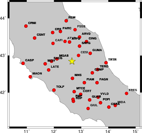
Waveform Inversion
The focal mechanism was determined using broadband seismic waveforms. The location of the event and the
and stations used for the waveform inversion are shown in the next figure.
|
|
Location of broadband stations used for waveform inversion
|
The program wvfgrd96 was used with good traces observed at short distance to determine the focal mechanism, depth and seismic moment. This technique requires a high quality signal and well determined velocity model for the Green functions. To the extent that these are the quality data, this type of mechanism should be preferred over the radiation pattern technique which requires the separate step of defining the pressure and tension quadrants and the correct strike.
The observed and predicted traces are filtered using the following gsac commands:
hp c 0.02 n 3
lp c 0.10 n 3
The results of this grid search from 0.5 to 19 km depth are as follow:
           DEPTH  STK   DIP  RAKE   MW    FIT
WVFGRD96    1.0   345    30   -90   3.87 0.3549
WVFGRD96    2.0   340    80   -90   4.01 0.4258
WVFGRD96    3.0   155    10   -95   3.99 0.5362
WVFGRD96    4.0   155    15   -95   3.97 0.5886
WVFGRD96    5.0   150    15  -100   4.08 0.6187
WVFGRD96    6.0   340    75   -90   4.08 0.6239
WVFGRD96    7.0   150    15  -100   4.07 0.6069
WVFGRD96    8.0   340    75   -80   4.02 0.5778
WVFGRD96    9.0   340    75   -80   4.02 0.5543
WVFGRD96   10.0   345    80   -80   4.02 0.5287
WVFGRD96   11.0   345    80   -80   4.03 0.5049
WVFGRD96   12.0   345    80   -80   4.03 0.4802
WVFGRD96   13.0   345    80   -80   4.03 0.4551
WVFGRD96   14.0   345    85   -80   4.04 0.4317
WVFGRD96   15.0   345    85   -80   4.08 0.4106
WVFGRD96   16.0   165    90    80   4.09 0.3847
WVFGRD96   17.0   165    85    75   4.10 0.3621
WVFGRD96   18.0   300    15    45   4.10 0.3412
WVFGRD96   19.0   310    15    55   4.11 0.3216
WVFGRD96   20.0   305    20    50   4.11 0.3031
WVFGRD96   21.0   310    20    55   4.11 0.2871
WVFGRD96   22.0   315    20    60   4.12 0.2722
WVFGRD96   23.0   310    25    55   4.12 0.2597
WVFGRD96   24.0   320    25    65   4.12 0.2497
WVFGRD96   25.0   330    30    75   4.12 0.2432
WVFGRD96   26.0   335    30    80   4.13 0.2393
WVFGRD96   27.0   325    30    70   4.13 0.2353
WVFGRD96   28.0   320    35    70   4.14 0.2300
WVFGRD96   29.0   165    70   -70   4.14 0.2246
The best solution is
WVFGRD96 6.0 340 75 -90 4.08 0.6239
The mechanism correspond to the best fit is
|
|
Figure 1. Waveform inversion focal mechanism
|
The best fit as a function of depth is given in the following figure:
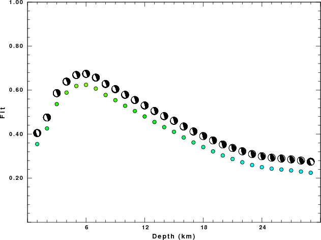
|
|
Figure 2. Depth sensitivity for waveform mechanism
|
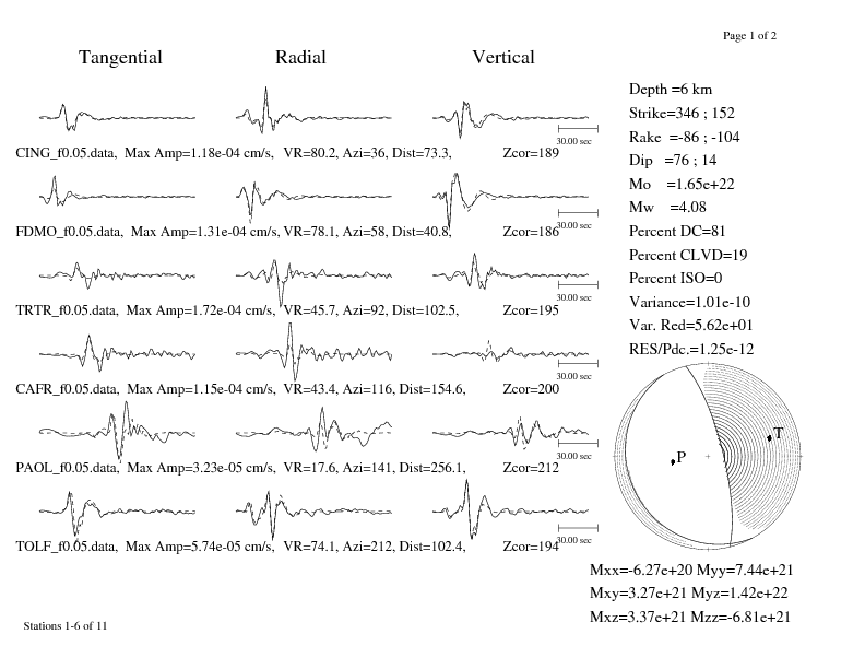
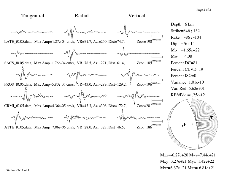
The comparison of the observed and predicted waveforms is given in the next figure. The red traces are the observed and the blue are the predicted.
Each observed-predicted component is plotted to the same scale and peak amplitudes are indicated by the numbers to the left of each trace. The number in black at the rightr of each predicted traces it the time shift required for maximum correlation between the observed and predicted traces. This time shift is required because the synthetics are not computed at exactly the same distance as the observed and because the velocity model used in the predictions may not be perfect.
A positive time shift indicates that the prediction is too fast and should be delayed to match the observed trace (shift to the right in this figure). A negative value indicates that the prediction is too slow.
The bandpass filter used in the processing and for the display was
hp c 0.02 n 3
lp c 0.10 n 3
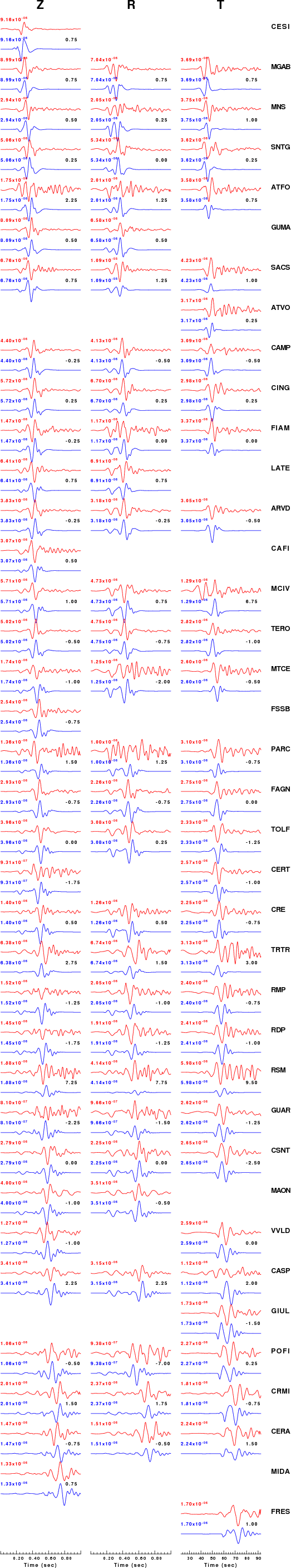
|
|
Figure 3. Waveform comparison for selected depth
|
|
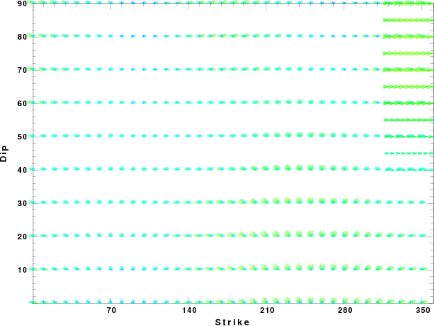
|
Focal mechanism sensitivity at the preferred depth. The red color indicates a very good fit to thewavefroms.
Each solution is plotted as a vector at a given value of strike and dip with the angle of the vector representing the rake angle, measured, with respect to the upward vertical (N) in the figure.
|
Discussion
Velocity Model
The nnCIA used for the waveform synthetic seismograms and for the surface wave eigenfunctions and dispersion is as follows:
MODEL.01
C.It. A. Di Luzio et al Earth Plan Lettrs 280 (2009) 1-12 Fig 5. 7-8 MODEL/SURF3
ISOTROPIC
KGS
FLAT EARTH
1-D
CONSTANT VELOCITY
LINE08
LINE09
LINE10
LINE11
      H(KM)   VP(KM/S)   VS(KM/S) RHO(GM/CC)         QP         QS       ETAP       ETAS      FREFP      FREFS
     1.5000     3.7497     2.1436     2.2753  0.500E-02  0.100E-01   0.00       0.00       1.00       1.00
     3.0000     4.9399     2.8210     2.4858  0.500E-02  0.100E-01   0.00       0.00       1.00       1.00
     3.0000     6.0129     3.4336     2.7058  0.500E-02  0.100E-01   0.00       0.00       1.00       1.00
     7.0000     5.5516     3.1475     2.6093  0.167E-02  0.333E-02   0.00       0.00       1.00       1.00
    15.0000     5.8805     3.3583     2.6770  0.167E-02  0.333E-02   0.00       0.00       1.00       1.00
     6.0000     7.1059     4.0081     3.0002  0.167E-02  0.333E-02   0.00       0.00       1.00       1.00
     8.0000     7.1000     3.9864     3.0120  0.167E-02  0.333E-02   0.00       0.00       1.00       1.00
     0.0000     7.9000     4.4036     3.2760  0.167E-02  0.333E-02   0.00       0.00       1.00       1.00
Quality Control
Here we tabulate the reasons for not using certain digital data sets
The following stations did not have a valid response files:
DATE=Sat Aug 28 07:48:21 CDT 2010
Last Changed 2010/08/28