2009/04/09 13:19:33 42.338 13.259 10.0 3.60 Italy
USGS Felt map for this earthquake
 USGS/SLU Moment Tensor Solution
 ENS  2009/04/09 13:19:33:0  42.34   13.26  10.0 3.6 Italy

 Stations used:
   IV.AOI IV.ASSB IV.BSSO IV.CAFR IV.CERA IV.CERT IV.CESI
   IV.CESX IV.CING IV.FAGN IV.FDMO IV.FIAM IV.GIUL IV.GUAR
   IV.INTR IV.LNSS IV.LPEL IV.MGAB IV.MIDA IV.MNS IV.MODR
   IV.MTCE IV.MURB IV.NRCA IV.OFFI IV.POFI IV.RDP IV.RNI2
   IV.SACS IV.SGG IV.TERO IV.TRIV IV.TRTR IV.VVLD MN.AQU

 Filtering commands used:
   hp c 0.02 n 3
   lp c 0.10 n 3

 Best Fitting Double Couple
  Mo = 6.10e+21 dyne-cm
  Mw = 3.79
  Z  = 9 km
  Plane   Strike  Dip  Rake
   NP1      330    50   -65
   NP2      114    46   -117
  Principal Axes:
   Axis    Value   Plunge  Azimuth
    T   6.10e+21      2      43
    N   0.00e+00     19     133
    P  -6.10e+21     71     307

 Moment Tensor: (dyne-cm)
    Component   Value
       Mxx     3.07e+21
       Mxy     3.34e+21
       Mxz    -9.54e+20
       Myy     2.37e+21
       Myz     1.66e+21
       Mzz    -5.44e+21


                     ##############
                 ----##################
              ------------############## T
             ----------------###########
           --------------------##############
          -----------------------#############
         -------------------------#############
        #---------------------------############
        ##-------------   -----------###########
       ###------------- P ------------###########
       ####------------   -------------##########
       #####---------------------------##########
       #######--------------------------#########
        #######-------------------------########
        ##########----------------------########
         ###########---------------------######
          ##############-----------------###--
           ###################---------#-----
             ###########################---
              #########################---
                 ######################
                     ##############


 Global CMT Convention Moment Tensor:
      R          T          P
 -5.44e+21  -9.54e+20  -1.66e+21
 -9.54e+20   3.07e+21  -3.34e+21
 -1.66e+21  -3.34e+21   2.37e+21


Details of the solution is found at

http://www.eas.slu.edu/eqc/eqc_mt/MECH.IT/20090409131933/index.html
|
      STK = 330
      DIP = 50
     RAKE = -65
       MW = 3.79
       HS = 9.0
The waveform inversion is preferred.
The following compares this source inversion to others
 USGS/SLU Moment Tensor Solution
 ENS  2009/04/09 13:19:33:0  42.34   13.26  10.0 3.6 Italy

 Stations used:
   IV.AOI IV.ASSB IV.BSSO IV.CAFR IV.CERA IV.CERT IV.CESI
   IV.CESX IV.CING IV.FAGN IV.FDMO IV.FIAM IV.GIUL IV.GUAR
   IV.INTR IV.LNSS IV.LPEL IV.MGAB IV.MIDA IV.MNS IV.MODR
   IV.MTCE IV.MURB IV.NRCA IV.OFFI IV.POFI IV.RDP IV.RNI2
   IV.SACS IV.SGG IV.TERO IV.TRIV IV.TRTR IV.VVLD MN.AQU

 Filtering commands used:
   hp c 0.02 n 3
   lp c 0.10 n 3

 Best Fitting Double Couple
  Mo = 6.10e+21 dyne-cm
  Mw = 3.79
  Z  = 9 km
  Plane   Strike  Dip  Rake
   NP1      330    50   -65
   NP2      114    46   -117
  Principal Axes:
   Axis    Value   Plunge  Azimuth
    T   6.10e+21      2      43
    N   0.00e+00     19     133
    P  -6.10e+21     71     307

 Moment Tensor: (dyne-cm)
    Component   Value
       Mxx     3.07e+21
       Mxy     3.34e+21
       Mxz    -9.54e+20
       Myy     2.37e+21
       Myz     1.66e+21
       Mzz    -5.44e+21


                     ##############
                 ----##################
              ------------############## T
             ----------------###########
           --------------------##############
          -----------------------#############
         -------------------------#############
        #---------------------------############
        ##-------------   -----------###########
       ###------------- P ------------###########
       ####------------   -------------##########
       #####---------------------------##########
       #######--------------------------#########
        #######-------------------------########
        ##########----------------------########
         ###########---------------------######
          ##############-----------------###--
           ###################---------#-----
             ###########################---
              #########################---
                 ######################
                     ##############


 Global CMT Convention Moment Tensor:
      R          T          P
 -5.44e+21  -9.54e+20  -1.66e+21
 -9.54e+20   3.07e+21  -3.34e+21
 -1.66e+21  -3.34e+21   2.37e+21


Details of the solution is found at

http://www.eas.slu.edu/eqc/eqc_mt/MECH.IT/20090409131933/index.html
|
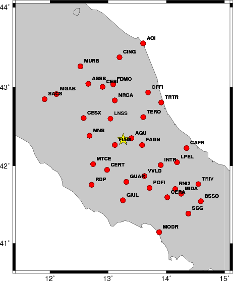
The focal mechanism was determined using broadband seismic waveforms. The location of the event and the and stations used for the waveform inversion are shown in the next figure.
|
|
|
|
The program wvfgrd96 was used with good traces observed at short distance to determine the focal mechanism, depth and seismic moment. This technique requires a high quality signal and well determined velocity model for the Green functions. To the extent that these are the quality data, this type of mechanism should be preferred over the radiation pattern technique which requires the separate step of defining the pressure and tension quadrants and the correct strike.
The observed and predicted traces are filtered using the following gsac commands:
hp c 0.02 n 3
lp c 0.10 n 3
The results of this grid search from 0.5 to 19 km depth are as follow:
           DEPTH  STK   DIP  RAKE   MW    FIT
WVFGRD96    0.5   310    50   -90   3.52 0.2705
WVFGRD96    1.0   125    45   -95   3.55 0.2519
WVFGRD96    2.0   345    45   -30   3.58 0.2464
WVFGRD96    3.0   350    35   -20   3.62 0.2746
WVFGRD96    4.0   345    40   -30   3.64 0.3102
WVFGRD96    5.0   340    35   -40   3.74 0.3414
WVFGRD96    6.0   330    40   -60   3.79 0.3968
WVFGRD96    7.0   325    45   -70   3.81 0.4464
WVFGRD96    8.0   325    45   -70   3.79 0.4681
WVFGRD96    9.0   330    50   -65   3.79 0.4720
WVFGRD96   10.0   335    50   -60   3.79 0.4670
WVFGRD96   11.0   335    50   -60   3.80 0.4565
WVFGRD96   12.0   335    50   -60   3.80 0.4425
WVFGRD96   13.0   340    50   -50   3.81 0.4286
WVFGRD96   14.0   345    50   -45   3.81 0.4137
WVFGRD96   15.0   345    50   -45   3.85 0.4086
WVFGRD96   16.0   345    50   -45   3.85 0.3957
WVFGRD96   17.0   345    55   -45   3.86 0.3821
WVFGRD96   18.0   345    60   -45   3.87 0.3693
WVFGRD96   19.0   345    60   -45   3.87 0.3581
WVFGRD96   20.0   345    60   -45   3.88 0.3473
WVFGRD96   21.0   345    55   -45   3.89 0.3377
WVFGRD96   22.0   345    55   -40   3.89 0.3299
WVFGRD96   23.0   345    55   -45   3.90 0.3231
WVFGRD96   24.0   345    55   -45   3.91 0.3162
WVFGRD96   25.0   350    60   -40   3.91 0.3085
WVFGRD96   26.0   350    60   -40   3.92 0.3011
WVFGRD96   27.0   345    55   -35   3.93 0.2937
WVFGRD96   28.0   345    55   -40   3.93 0.2857
WVFGRD96   29.0   345    55   -40   3.94 0.2756
The best solution is
WVFGRD96 9.0 330 50 -65 3.79 0.4720
The mechanism correspond to the best fit is
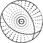
|
|
|
The best fit as a function of depth is given in the following figure:
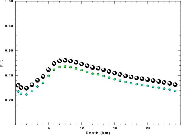
|
|
|
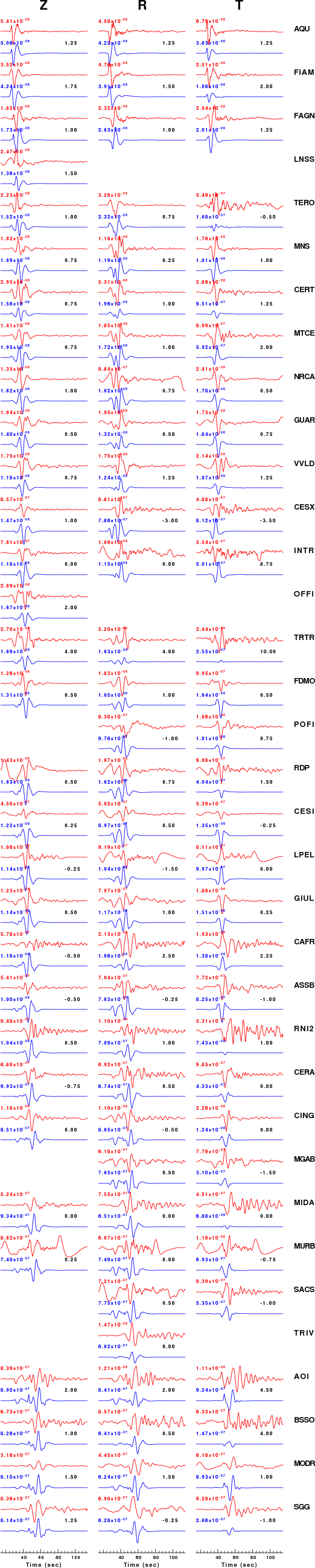
The comparison of the observed and predicted waveforms is given in the next figure. The red traces are the observed and the blue are the predicted. Each observed-predicted component is plotted to the same scale and peak amplitudes are indicated by the numbers to the left of each trace. The number in black at the rightr of each predicted traces it the time shift required for maximum correlation between the observed and predicted traces. This time shift is required because the synthetics are not computed at exactly the same distance as the observed and because the velocity model used in the predictions may not be perfect. A positive time shift indicates that the prediction is too fast and should be delayed to match the observed trace (shift to the right in this figure). A negative value indicates that the prediction is too slow. The bandpass filter used in the processing and for the display was
hp c 0.02 n 3
lp c 0.10 n 3
|
|
|
|
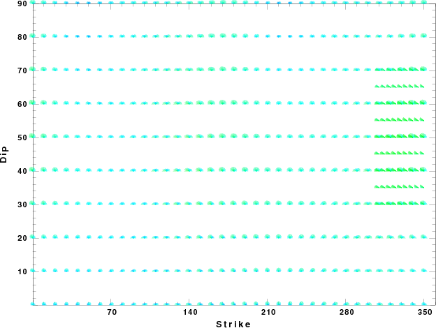
| Focal mechanism sensitivity at the preferred depth. The red color indicates a very good fit to thewavefroms. Each solution is plotted as a vector at a given value of strike and dip with the angle of the vector representing the rake angle, measured, with respect to the upward vertical (N) in the figure. |
The nnCIA used for the waveform synthetic seismograms and for the surface wave eigenfunctions and dispersion is as follows:
MODEL.01
C.It. A. Di Luzio et al Earth Plan Lettrs 280 (2009) 1-12 Fig 5. 7-8 MODEL/SURF3
ISOTROPIC
KGS
FLAT EARTH
1-D
CONSTANT VELOCITY
LINE08
LINE09
LINE10
LINE11
      H(KM)   VP(KM/S)   VS(KM/S) RHO(GM/CC)         QP         QS       ETAP       ETAS      FREFP      FREFS
     1.5000     3.7497     2.1436     2.2753  0.500E-02  0.100E-01   0.00       0.00       1.00       1.00
     3.0000     4.9399     2.8210     2.4858  0.500E-02  0.100E-01   0.00       0.00       1.00       1.00
     3.0000     6.0129     3.4336     2.7058  0.500E-02  0.100E-01   0.00       0.00       1.00       1.00
     7.0000     5.5516     3.1475     2.6093  0.167E-02  0.333E-02   0.00       0.00       1.00       1.00
    15.0000     5.8805     3.3583     2.6770  0.167E-02  0.333E-02   0.00       0.00       1.00       1.00
     6.0000     7.1059     4.0081     3.0002  0.167E-02  0.333E-02   0.00       0.00       1.00       1.00
     8.0000     7.1000     3.9864     3.0120  0.167E-02  0.333E-02   0.00       0.00       1.00       1.00
     0.0000     7.9000     4.4036     3.2760  0.167E-02  0.333E-02   0.00       0.00       1.00       1.00
Here we tabulate the reasons for not using certain digital data sets
The following stations did not have a valid response files:
DATE=Mon Apr 20 10:42:20 CDT 2009