2009/04/09 03:14:52 42.338 13.437 18.0 4.20 Italy
USGS Felt map for this earthquake
 USGS/SLU Moment Tensor Solution
 ENS  2009/04/09 03:14:52:0  42.34   13.44  18.0 4.2 Italy

 Stations used:
   IV.ARVD IV.ASSB IV.CAFE IV.CAFR IV.CAMP IV.CASP IV.CERA
   IV.CERT IV.CESX IV.CING IV.CSNT IV.FDMO IV.FRES IV.INTR
   IV.LATE IV.LNSS IV.MAON IV.MGAB IV.MIDA IV.MSAG IV.MTCE
   IV.MURB IV.NRCA IV.OFFI IV.PARC IV.PESA IV.POFI IV.PTRJ
   IV.RDP IV.ROM9 IV.RSM IV.SACS IV.SGRT IV.TERO IV.TOLF
   IV.TRTR IV.VAGA IV.VVLD

 Filtering commands used:
   hp c 0.02 n 3
   lp c 0.10 n 3

 Best Fitting Double Couple
  Mo = 3.94e+22 dyne-cm
  Mw = 4.33
  Z  = 16 km
  Plane   Strike  Dip  Rake
   NP1      330    85   -55
   NP2       67    35   -171
  Principal Axes:
   Axis    Value   Plunge  Azimuth
    T   3.94e+22     31      32
    N   0.00e+00     35     146
    P  -3.94e+22     40     272

 Moment Tensor: (dyne-cm)
    Component   Value
       Mxx     2.09e+22
       Mxy     1.37e+22
       Mxz     1.42e+22
       Myy    -1.53e+22
       Myz     2.85e+22
       Mzz    -5.60e+21


                     ##############
                 -#####################
              -----#######################
             --------#############   ######
           -----------############ T ########
          -------------###########   #########
         ---------------#######################
        ------------------#####################-
        -------------------####################-
       -------   -----------###################--
       ------- P ------------#################---
       -------   -------------###############----
       ------------------------#############-----
        ------------------------###########-----
        -------------------------#########------
         -------------------------######-------
          #------------------------##---------
           ###--------------------##---------
             ######----------########------
              #######################-----
                 #####################-
                     ##############


 Global CMT Convention Moment Tensor:
      R          T          P
 -5.60e+21   1.42e+22  -2.85e+22
  1.42e+22   2.09e+22  -1.37e+22
 -2.85e+22  -1.37e+22  -1.53e+22


Details of the solution is found at

http://www.eas.slu.edu/eqc/eqc_mt/MECH.IT/20090409031452/index.html
|
      STK = 330
      DIP = 85
     RAKE = -55
       MW = 4.33
       HS = 16.0
The waveform inversion is preferred.
The following compares this source inversion to others
 USGS/SLU Moment Tensor Solution
 ENS  2009/04/09 03:14:52:0  42.34   13.44  18.0 4.2 Italy

 Stations used:
   IV.ARVD IV.ASSB IV.CAFE IV.CAFR IV.CAMP IV.CASP IV.CERA
   IV.CERT IV.CESX IV.CING IV.CSNT IV.FDMO IV.FRES IV.INTR
   IV.LATE IV.LNSS IV.MAON IV.MGAB IV.MIDA IV.MSAG IV.MTCE
   IV.MURB IV.NRCA IV.OFFI IV.PARC IV.PESA IV.POFI IV.PTRJ
   IV.RDP IV.ROM9 IV.RSM IV.SACS IV.SGRT IV.TERO IV.TOLF
   IV.TRTR IV.VAGA IV.VVLD

 Filtering commands used:
   hp c 0.02 n 3
   lp c 0.10 n 3

 Best Fitting Double Couple
  Mo = 3.94e+22 dyne-cm
  Mw = 4.33
  Z  = 16 km
  Plane   Strike  Dip  Rake
   NP1      330    85   -55
   NP2       67    35   -171
  Principal Axes:
   Axis    Value   Plunge  Azimuth
    T   3.94e+22     31      32
    N   0.00e+00     35     146
    P  -3.94e+22     40     272

 Moment Tensor: (dyne-cm)
    Component   Value
       Mxx     2.09e+22
       Mxy     1.37e+22
       Mxz     1.42e+22
       Myy    -1.53e+22
       Myz     2.85e+22
       Mzz    -5.60e+21


                     ##############
                 -#####################
              -----#######################
             --------#############   ######
           -----------############ T ########
          -------------###########   #########
         ---------------#######################
        ------------------#####################-
        -------------------####################-
       -------   -----------###################--
       ------- P ------------#################---
       -------   -------------###############----
       ------------------------#############-----
        ------------------------###########-----
        -------------------------#########------
         -------------------------######-------
          #------------------------##---------
           ###--------------------##---------
             ######----------########------
              #######################-----
                 #####################-
                     ##############


 Global CMT Convention Moment Tensor:
      R          T          P
 -5.60e+21   1.42e+22  -2.85e+22
  1.42e+22   2.09e+22  -1.37e+22
 -2.85e+22  -1.37e+22  -1.53e+22


Details of the solution is found at

http://www.eas.slu.edu/eqc/eqc_mt/MECH.IT/20090409031452/index.html
|
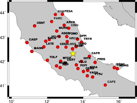
The focal mechanism was determined using broadband seismic waveforms. The location of the event and the and stations used for the waveform inversion are shown in the next figure.
|
|
|
|
The program wvfgrd96 was used with good traces observed at short distance to determine the focal mechanism, depth and seismic moment. This technique requires a high quality signal and well determined velocity model for the Green functions. To the extent that these are the quality data, this type of mechanism should be preferred over the radiation pattern technique which requires the separate step of defining the pressure and tension quadrants and the correct strike.
The observed and predicted traces are filtered using the following gsac commands:
hp c 0.02 n 3
lp c 0.10 n 3
The results of this grid search from 0.5 to 19 km depth are as follow:
           DEPTH  STK   DIP  RAKE   MW    FIT
WVFGRD96    0.5   120    45   -95   3.82 0.2438
WVFGRD96    1.0   300    45   -90   3.81 0.1903
WVFGRD96    2.0   120    45   -90   3.99 0.2675
WVFGRD96    3.0   150    80   -60   3.99 0.2421
WVFGRD96    4.0   155    85   -60   4.03 0.2923
WVFGRD96    5.0   150    85   -65   4.05 0.3315
WVFGRD96    6.0   150    90    60   4.07 0.3651
WVFGRD96    7.0   150    90    55   4.09 0.3993
WVFGRD96    8.0   150    90    60   4.18 0.4252
WVFGRD96    9.0   150    90    60   4.20 0.4558
WVFGRD96   10.0   150    90    60   4.22 0.4793
WVFGRD96   11.0   150    90    55   4.24 0.4976
WVFGRD96   12.0   330    90   -55   4.26 0.5125
WVFGRD96   13.0   150    90    55   4.28 0.5229
WVFGRD96   14.0   330    85   -55   4.30 0.5316
WVFGRD96   15.0   150    90    55   4.31 0.5333
WVFGRD96   16.0   330    85   -55   4.33 0.5379
WVFGRD96   17.0   330    85   -55   4.34 0.5368
WVFGRD96   18.0   330    85   -55   4.35 0.5334
WVFGRD96   19.0   330    80   -55   4.37 0.5284
WVFGRD96   20.0   330    80   -55   4.38 0.5225
WVFGRD96   21.0   330    80   -55   4.39 0.5139
WVFGRD96   22.0   330    80   -55   4.40 0.5041
WVFGRD96   23.0   330    80   -55   4.41 0.4931
WVFGRD96   24.0   330    80   -60   4.41 0.4808
WVFGRD96   25.0   330    85   -60   4.42 0.4683
WVFGRD96   26.0   330    85   -60   4.42 0.4554
WVFGRD96   27.0   330    85   -60   4.43 0.4417
WVFGRD96   28.0   155    90    60   4.43 0.4249
WVFGRD96   29.0   150    90    60   4.43 0.4116
The best solution is
WVFGRD96 16.0 330 85 -55 4.33 0.5379
The mechanism correspond to the best fit is
|
|
|
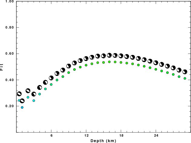
The best fit as a function of depth is given in the following figure:
|
|
|
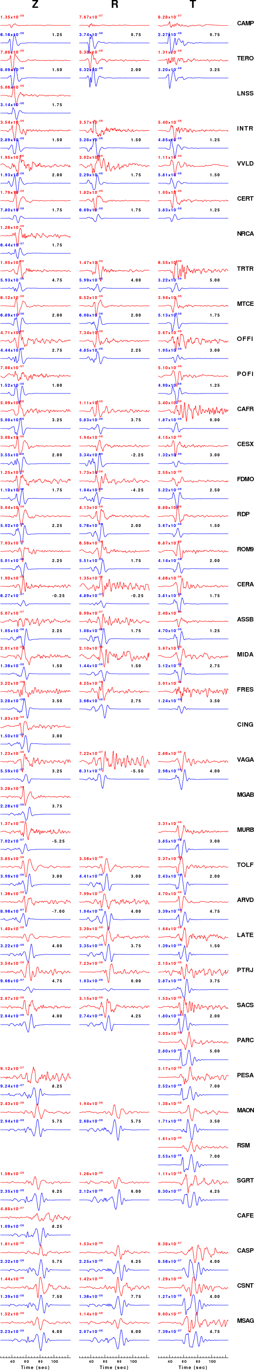
The comparison of the observed and predicted waveforms is given in the next figure. The red traces are the observed and the blue are the predicted. Each observed-predicted component is plotted to the same scale and peak amplitudes are indicated by the numbers to the left of each trace. The number in black at the rightr of each predicted traces it the time shift required for maximum correlation between the observed and predicted traces. This time shift is required because the synthetics are not computed at exactly the same distance as the observed and because the velocity model used in the predictions may not be perfect. A positive time shift indicates that the prediction is too fast and should be delayed to match the observed trace (shift to the right in this figure). A negative value indicates that the prediction is too slow. The bandpass filter used in the processing and for the display was
hp c 0.02 n 3
lp c 0.10 n 3
|
|
|
|
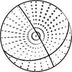
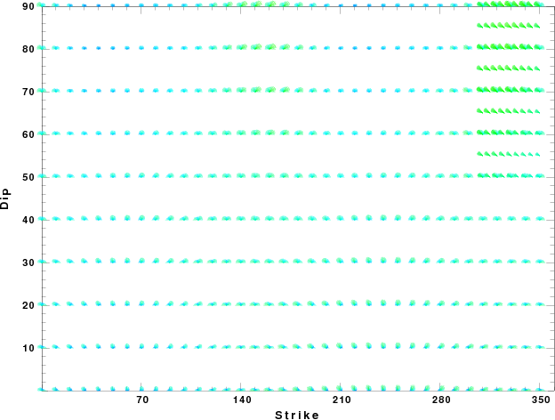
| Focal mechanism sensitivity at the preferred depth. The red color indicates a very good fit to thewavefroms. Each solution is plotted as a vector at a given value of strike and dip with the angle of the vector representing the rake angle, measured, with respect to the upward vertical (N) in the figure. |
The WUS used for the waveform synthetic seismograms and for the surface wave eigenfunctions and dispersion is as follows:
MODEL.01
Model after     8 iterations
ISOTROPIC
KGS
FLAT EARTH
1-D
CONSTANT VELOCITY
LINE08
LINE09
LINE10
LINE11
      H(KM)   VP(KM/S)   VS(KM/S) RHO(GM/CC)         QP         QS       ETAP       ETAS      FREFP      FREFS
     1.9000     3.4065     2.0089     2.2150  0.302E-02  0.679E-02   0.00       0.00       1.00       1.00
     6.1000     5.5445     3.2953     2.6089  0.349E-02  0.784E-02   0.00       0.00       1.00       1.00
    13.0000     6.2708     3.7396     2.7812  0.212E-02  0.476E-02   0.00       0.00       1.00       1.00
    19.0000     6.4075     3.7680     2.8223  0.111E-02  0.249E-02   0.00       0.00       1.00       1.00
     0.0000     7.9000     4.6200     3.2760  0.164E-10  0.370E-10   0.00       0.00       1.00       1.00
Here we tabulate the reasons for not using certain digital data sets
The following stations did not have a valid response files:
DATE=Wed Apr 15 20:01:12 CDT 2009