2009/04/07 09:26:28 42.342 13.388 10.0 4.70 Italy
USGS Felt map for this earthquake
 USGS/SLU Moment Tensor Solution
 ENS  2009/04/07 09:26:28:0  42.34   13.39  10.0 4.7 Italy

 Stations used:
   IV.AOI IV.ARCI IV.ARVD IV.BSSO IV.CAFI IV.CAFR IV.CAMP
   IV.CERA IV.CESI IV.CING IV.FDMO IV.FSSB IV.GIUL IV.INTR
   IV.MA9 IV.MGAB IV.MIDA IV.MNS IV.MODR IV.PESA IV.PIEI
   IV.POFI IV.RNI2 IV.SACS IV.SGG IV.TERO IV.TOLF IV.TRIV
   IV.TRTR IV.VAGA

 Filtering commands used:
   hp c 0.02 n 3
   lp c 0.10 n 3

 Best Fitting Double Couple
  Mo = 2.54e+23 dyne-cm
  Mw = 4.87
  Z  = 12 km
  Plane   Strike  Dip  Rake
   NP1      146    64   -106
   NP2        0    30   -60
  Principal Axes:
   Axis    Value   Plunge  Azimuth
    T   2.54e+23     18     248
    N   0.00e+00     14     153
    P  -2.54e+23     67      27

 Moment Tensor: (dyne-cm)
    Component   Value
       Mxx     0.00e+00
       Mxy     6.35e+22
       Mxz    -1.10e+23
       Myy     1.91e+23
       Myz    -1.10e+23
       Mzz    -1.91e+23


                     ----------####
                 -----------------#####
              ##--------------------######
             ###----------------------#####
           #####-----------------------######
          #######-----------------------######
         ########------------------------######
        ##########-----------   ----------######
        ##########----------- P ----------######
       ############----------   -----------######
       #############-----------------------######
       ##############----------------------######
       ###############---------------------######
        ##   ##########-------------------######
        ## T ############-----------------######
         #   #############---------------######
          ##################------------######
           ###################---------######
             ###################------#####
              #####################-######
                 #################-----
                     ##########----


 Global CMT Convention Moment Tensor:
      R          T          P
 -1.91e+23  -1.10e+23   1.10e+23
 -1.10e+23   0.00e+00  -6.35e+22
  1.10e+23  -6.35e+22   1.91e+23


Details of the solution is found at

http://www.eas.slu.edu/eqc/eqc_mt/MECH.IT/20090407092628/index.html
|
      STK = 0
      DIP = 30
     RAKE = -60
       MW = 4.87
       HS = 12.0
The waveform inversion is preferred.
The following compares this source inversion to others
 USGS/SLU Moment Tensor Solution
 ENS  2009/04/07 09:26:28:0  42.34   13.39  10.0 4.7 Italy

 Stations used:
   IV.AOI IV.ARCI IV.ARVD IV.BSSO IV.CAFI IV.CAFR IV.CAMP
   IV.CERA IV.CESI IV.CING IV.FDMO IV.FSSB IV.GIUL IV.INTR
   IV.MA9 IV.MGAB IV.MIDA IV.MNS IV.MODR IV.PESA IV.PIEI
   IV.POFI IV.RNI2 IV.SACS IV.SGG IV.TERO IV.TOLF IV.TRIV
   IV.TRTR IV.VAGA

 Filtering commands used:
   hp c 0.02 n 3
   lp c 0.10 n 3

 Best Fitting Double Couple
  Mo = 2.54e+23 dyne-cm
  Mw = 4.87
  Z  = 12 km
  Plane   Strike  Dip  Rake
   NP1      146    64   -106
   NP2        0    30   -60
  Principal Axes:
   Axis    Value   Plunge  Azimuth
    T   2.54e+23     18     248
    N   0.00e+00     14     153
    P  -2.54e+23     67      27

 Moment Tensor: (dyne-cm)
    Component   Value
       Mxx     0.00e+00
       Mxy     6.35e+22
       Mxz    -1.10e+23
       Myy     1.91e+23
       Myz    -1.10e+23
       Mzz    -1.91e+23


                     ----------####
                 -----------------#####
              ##--------------------######
             ###----------------------#####
           #####-----------------------######
          #######-----------------------######
         ########------------------------######
        ##########-----------   ----------######
        ##########----------- P ----------######
       ############----------   -----------######
       #############-----------------------######
       ##############----------------------######
       ###############---------------------######
        ##   ##########-------------------######
        ## T ############-----------------######
         #   #############---------------######
          ##################------------######
           ###################---------######
             ###################------#####
              #####################-######
                 #################-----
                     ##########----


 Global CMT Convention Moment Tensor:
      R          T          P
 -1.91e+23  -1.10e+23   1.10e+23
 -1.10e+23   0.00e+00  -6.35e+22
  1.10e+23  -6.35e+22   1.91e+23


Details of the solution is found at

http://www.eas.slu.edu/eqc/eqc_mt/MECH.IT/20090407092628/index.html
|
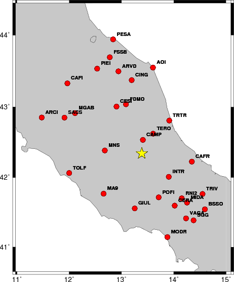
The focal mechanism was determined using broadband seismic waveforms. The location of the event and the and stations used for the waveform inversion are shown in the next figure.
|
|
|
|
The program wvfgrd96 was used with good traces observed at short distance to determine the focal mechanism, depth and seismic moment. This technique requires a high quality signal and well determined velocity model for the Green functions. To the extent that these are the quality data, this type of mechanism should be preferred over the radiation pattern technique which requires the separate step of defining the pressure and tension quadrants and the correct strike.
The observed and predicted traces are filtered using the following gsac commands:
hp c 0.02 n 3
lp c 0.10 n 3
The results of this grid search from 0.5 to 19 km depth are as follow:
           DEPTH  STK   DIP  RAKE   MW    FIT
WVFGRD96    0.5   330    40    90   4.46 0.2087
WVFGRD96    1.0   330    40    85   4.45 0.1626
WVFGRD96    2.0   155    50    95   4.62 0.2300
WVFGRD96    3.0   300    30    40   4.63 0.2128
WVFGRD96    4.0   345    20   105   4.68 0.2513
WVFGRD96    5.0   145    70    80   4.70 0.2847
WVFGRD96    6.0   145    70    75   4.71 0.3080
WVFGRD96    7.0   145    70    75   4.72 0.3222
WVFGRD96    8.0   145    70    75   4.80 0.3371
WVFGRD96    9.0   -10    25   -70   4.83 0.3501
WVFGRD96   10.0   350    25   -70   4.84 0.3592
WVFGRD96   11.0     0    30   -60   4.85 0.3642
WVFGRD96   12.0     0    30   -60   4.87 0.3661
WVFGRD96   13.0     0    30   -60   4.88 0.3641
WVFGRD96   14.0     5    30   -50   4.89 0.3595
WVFGRD96   15.0     5    30   -50   4.90 0.3533
WVFGRD96   16.0     5    30   -50   4.91 0.3457
WVFGRD96   17.0     5    30   -50   4.92 0.3366
WVFGRD96   18.0     5    30   -50   4.93 0.3264
WVFGRD96   19.0    10    35   -40   4.93 0.3172
WVFGRD96   20.0    15    40   -30   4.93 0.3080
WVFGRD96   21.0     5    40   -40   4.95 0.3024
WVFGRD96   22.0     5    40   -40   4.96 0.2954
WVFGRD96   23.0     5    45   -35   4.96 0.2883
WVFGRD96   24.0     5    45   -35   4.97 0.2811
WVFGRD96   25.0     5    45   -35   4.98 0.2740
WVFGRD96   26.0     5    45   -35   4.98 0.2666
WVFGRD96   27.0     5    45   -35   4.99 0.2597
WVFGRD96   28.0     5    45   -30   4.99 0.2529
WVFGRD96   29.0     5    45   -30   5.00 0.2462
The best solution is
WVFGRD96 12.0 0 30 -60 4.87 0.3661
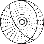
The mechanism correspond to the best fit is
|
|
|
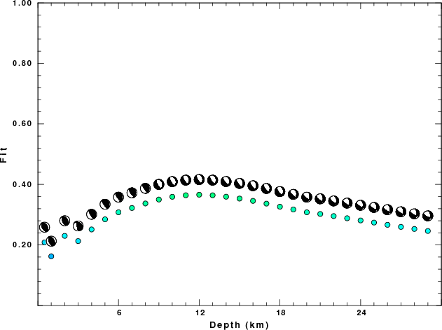
The best fit as a function of depth is given in the following figure:
|
|
|
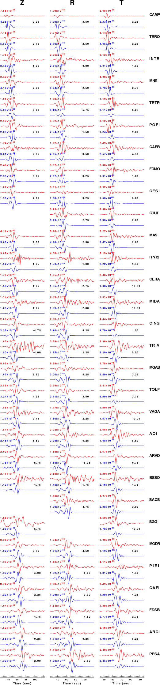
The comparison of the observed and predicted waveforms is given in the next figure. The red traces are the observed and the blue are the predicted. Each observed-predicted component is plotted to the same scale and peak amplitudes are indicated by the numbers to the left of each trace. The number in black at the rightr of each predicted traces it the time shift required for maximum correlation between the observed and predicted traces. This time shift is required because the synthetics are not computed at exactly the same distance as the observed and because the velocity model used in the predictions may not be perfect. A positive time shift indicates that the prediction is too fast and should be delayed to match the observed trace (shift to the right in this figure). A negative value indicates that the prediction is too slow. The bandpass filter used in the processing and for the display was
hp c 0.02 n 3
lp c 0.10 n 3
|
|
|
|
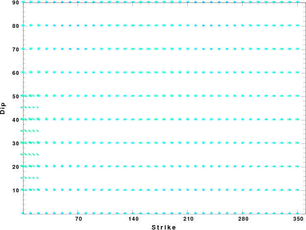
| Focal mechanism sensitivity at the preferred depth. The red color indicates a very good fit to thewavefroms. Each solution is plotted as a vector at a given value of strike and dip with the angle of the vector representing the rake angle, measured, with respect to the upward vertical (N) in the figure. |
The WUS used for the waveform synthetic seismograms and for the surface wave eigenfunctions and dispersion is as follows:
MODEL.01
Model after     8 iterations
ISOTROPIC
KGS
FLAT EARTH
1-D
CONSTANT VELOCITY
LINE08
LINE09
LINE10
LINE11
      H(KM)   VP(KM/S)   VS(KM/S) RHO(GM/CC)         QP         QS       ETAP       ETAS      FREFP      FREFS
     1.9000     3.4065     2.0089     2.2150  0.302E-02  0.679E-02   0.00       0.00       1.00       1.00
     6.1000     5.5445     3.2953     2.6089  0.349E-02  0.784E-02   0.00       0.00       1.00       1.00
    13.0000     6.2708     3.7396     2.7812  0.212E-02  0.476E-02   0.00       0.00       1.00       1.00
    19.0000     6.4075     3.7680     2.8223  0.111E-02  0.249E-02   0.00       0.00       1.00       1.00
     0.0000     7.9000     4.6200     3.2760  0.164E-10  0.370E-10   0.00       0.00       1.00       1.00
Here we tabulate the reasons for not using certain digital data sets
The following stations did not have a valid response files:
DATE=Thu Apr 16 11:15:41 CDT 2009