Location
Location ANSS
2022/09/10 15:58:13 47.68 7.48 10.0 4.7 FR/SW/DE
Focal Mechanism
 USGS/SLU Moment Tensor Solution
 ENS  2022/09/10 15:58:13:6  47.68    7.48  10.0 4.7 FR/SW/DE

 Stations used:
   BW.ALFT BW.BGDS BW.BHG BW.FFB1 BW.FFB2 BW.FFB3 BW.HROE
   BW.KW1 BW.MGS01 BW.MGSBH BW.OBER BW.PART BW.RJOB BW.RNON
   BW.RTBE BW.TON CH.ACB CH.AIGLE CH.BALST CH.BAULM CH.BERNI
   CH.BNALP CH.BOURR CH.BRANT CH.CHAMB CH.COLLE CH.DAVOX
   CH.DIX CH.EMMET CH.FIESA CH.FULLY CH.FUORN CH.FUSIO
   CH.GIMEL CH.GRIMS CH.GRYON CH.HASLI CH.ILLEZ CH.JAUN
   CH.LADOL CH.LAUCH CH.LIENZ CH.LKBD2 CH.LLS CH.METMA
   CH.MFERR CH.MMK CH.MUO CH.MUTEZ CH.NALPS CH.PANIX CH.PLONS
   CH.ROMAN CH.SAIRA CH.SALAN CH.SAVIG CH.SENIN CH.SIMPL
   CH.SLE CH.TORNY CH.VANNI CH.VDL CH.VDR CH.VINZL CH.VMV
   CH.WEIN2 CH.WGT CH.WIMIS CH.WOLEN GE.STU GE.WLF MN.BNI
   OE.ABTA OE.DAVA OE.FETA OE.MOTA OE.RETA OE.SQTA OE.WATA
   OE.WTTA OX.MLN TH.SPAHL

 Filtering commands used:
   cut o DIST/3.3 -30 o DIST/3.3 +70
   rtr
   taper w 0.1
   hp c 0.03 n 3
   lp c 0.06 n 3

 Best Fitting Double Couple
  Mo = 7.50e+21 dyne-cm
  Mw = 3.85
  Z  = 13 km
  Plane   Strike  Dip  Rake
   NP1      100    90   -165
   NP2       10    75     0
  Principal Axes:
   Axis    Value   Plunge  Azimuth
    T   7.50e+21     11     234
    N   0.00e+00     75     100
    P  -7.50e+21     11     326

 Moment Tensor: (dyne-cm)
    Component   Value
       Mxx    -2.48e+21
       Mxy     6.81e+21
       Mxz    -1.91e+21
       Myy     2.48e+21
       Myz    -3.37e+20
       Mzz     0.00e+00


                     -----------###
                   -------------#######
              -- P --------------#########
             ---   --------------##########
           ----------------------############
          -----------------------#############
         ------------------------##############
        -------------------------###############
        -------------------------###############
       #####--------------------#################
       ################---------#################
       #########################-################
       ########################-------------#####
        #######################-----------------
        #######################-----------------
         ##   ################-----------------
          # T ###############-----------------
              ###############----------------
             ###############---------------
              #############---------------
                 #########-------------
                     ####----------


 Global CMT Convention Moment Tensor:
      R          T          P
  0.00e+00  -1.91e+21   3.37e+20
 -1.91e+21  -2.48e+21  -6.81e+21
  3.37e+20  -6.81e+21   2.48e+21


Details of the solution is found at

http://www.eas.slu.edu/eqc/eqc_mt/MECH.NA/20220910155813/index.html
|
Preferred Solution
The preferred solution from an analysis of the surface-wave spectral amplitude radiation pattern, waveform inversion and first motion observations is
      STK = 10
      DIP = 75
     RAKE = 0
       MW = 3.85
       HS = 13.0
The NDK file is 20220910155813.ndk
The waveform inversion is preferred.
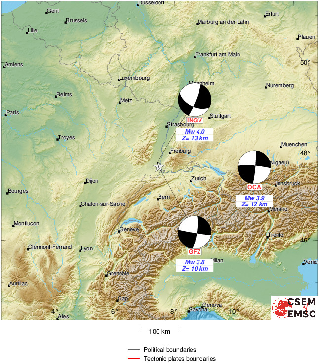
Moment Tensor Comparison
The following compares this source inversion to others
| SLU |
OTHER |
 USGS/SLU Moment Tensor Solution
 ENS  2022/09/10 15:58:13:6  47.68    7.48  10.0 4.7 FR/SW/DE

 Stations used:
   BW.ALFT BW.BGDS BW.BHG BW.FFB1 BW.FFB2 BW.FFB3 BW.HROE
   BW.KW1 BW.MGS01 BW.MGSBH BW.OBER BW.PART BW.RJOB BW.RNON
   BW.RTBE BW.TON CH.ACB CH.AIGLE CH.BALST CH.BAULM CH.BERNI
   CH.BNALP CH.BOURR CH.BRANT CH.CHAMB CH.COLLE CH.DAVOX
   CH.DIX CH.EMMET CH.FIESA CH.FULLY CH.FUORN CH.FUSIO
   CH.GIMEL CH.GRIMS CH.GRYON CH.HASLI CH.ILLEZ CH.JAUN
   CH.LADOL CH.LAUCH CH.LIENZ CH.LKBD2 CH.LLS CH.METMA
   CH.MFERR CH.MMK CH.MUO CH.MUTEZ CH.NALPS CH.PANIX CH.PLONS
   CH.ROMAN CH.SAIRA CH.SALAN CH.SAVIG CH.SENIN CH.SIMPL
   CH.SLE CH.TORNY CH.VANNI CH.VDL CH.VDR CH.VINZL CH.VMV
   CH.WEIN2 CH.WGT CH.WIMIS CH.WOLEN GE.STU GE.WLF MN.BNI
   OE.ABTA OE.DAVA OE.FETA OE.MOTA OE.RETA OE.SQTA OE.WATA
   OE.WTTA OX.MLN TH.SPAHL

 Filtering commands used:
   cut o DIST/3.3 -30 o DIST/3.3 +70
   rtr
   taper w 0.1
   hp c 0.03 n 3
   lp c 0.06 n 3

 Best Fitting Double Couple
  Mo = 7.50e+21 dyne-cm
  Mw = 3.85
  Z  = 13 km
  Plane   Strike  Dip  Rake
   NP1      100    90   -165
   NP2       10    75     0
  Principal Axes:
   Axis    Value   Plunge  Azimuth
    T   7.50e+21     11     234
    N   0.00e+00     75     100
    P  -7.50e+21     11     326

 Moment Tensor: (dyne-cm)
    Component   Value
       Mxx    -2.48e+21
       Mxy     6.81e+21
       Mxz    -1.91e+21
       Myy     2.48e+21
       Myz    -3.37e+20
       Mzz     0.00e+00


                     -----------###
                   -------------#######
              -- P --------------#########
             ---   --------------##########
           ----------------------############
          -----------------------#############
         ------------------------##############
        -------------------------###############
        -------------------------###############
       #####--------------------#################
       ################---------#################
       #########################-################
       ########################-------------#####
        #######################-----------------
        #######################-----------------
         ##   ################-----------------
          # T ###############-----------------
              ###############----------------
             ###############---------------
              #############---------------
                 #########-------------
                     ####----------


 Global CMT Convention Moment Tensor:
      R          T          P
  0.00e+00  -1.91e+21   3.37e+20
 -1.91e+21  -2.48e+21  -6.81e+21
  3.37e+20  -6.81e+21   2.48e+21


Details of the solution is found at

http://www.eas.slu.edu/eqc/eqc_mt/MECH.NA/20220910155813/index.html
|
EMSC-CSEM Summary
|
Magnitudes
ML Magnitude
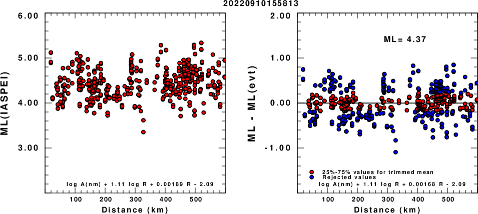
(a) ML computed using the IASPEI formula for Horizontal components; (b) ML residuals computed using a modified IASPEI formula that accounts for path specific attenuation; the values used for the trimmed mean are indicated. The ML relation used for each figure is given at the bottom of each plot.
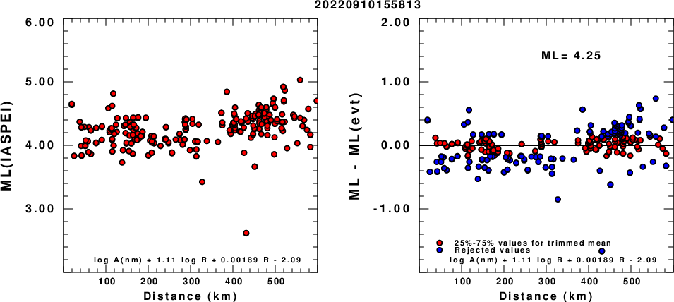
(a) ML computed using the IASPEI formula for Vertical components (research); (b) ML residuals computed using a modified IASPEI formula that accounts for path specific attenuation; the values used for the trimmed mean are indicated. The ML relation used for each figure is given at the bottom of each plot.
Context
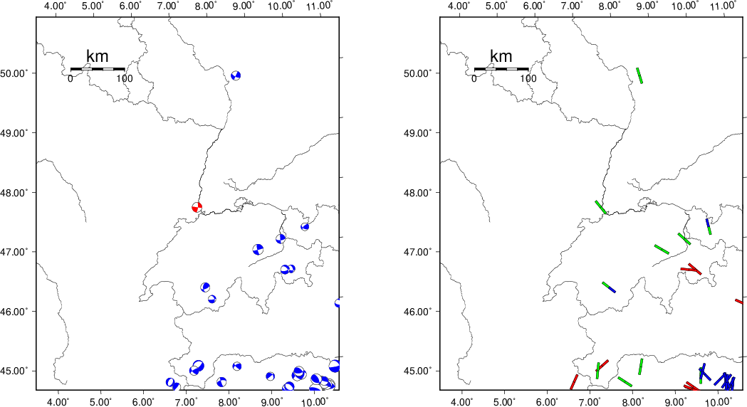
The next figure presents the focal mechanism for this earthquake (red) in the context of other events (blue) in the SLU Moment Tensor Catalog which are within ± 0.5 degrees of the new event. This comparison is shown in the left panel of the figure. The right panel shows the inferred direction of maximum compressive stress and the type of faulting (green is strike-slip, red is normal, blue is thrust; oblique is shown by a combination of colors).
Waveform Inversion
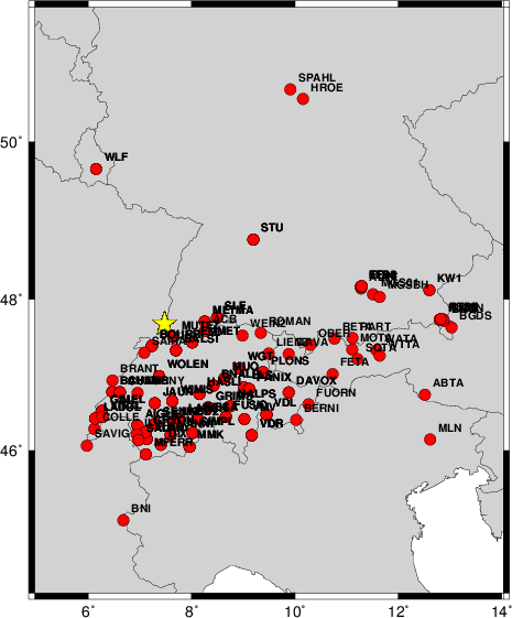
The focal mechanism was determined using broadband seismic waveforms. The location of the event and the
and stations used for the waveform inversion are shown in the next figure.
|
|
Location of broadband stations used for waveform inversion
|
The program wvfgrd96 was used with good traces observed at short distance to determine the focal mechanism, depth and seismic moment. This technique requires a high quality signal and well determined velocity model for the Green functions. To the extent that these are the quality data, this type of mechanism should be preferred over the radiation pattern technique which requires the separate step of defining the pressure and tension quadrants and the correct strike.
The observed and predicted traces are filtered using the following gsac commands:
cut o DIST/3.3 -30 o DIST/3.3 +70
rtr
taper w 0.1
hp c 0.03 n 3
lp c 0.06 n 3
The results of this grid search from 0.5 to 19 km depth are as follow:
           DEPTH  STK   DIP  RAKE   MW    FIT
WVFGRD96    1.0    15    90    -5   3.46 0.3923
WVFGRD96    2.0    10    75   -15   3.59 0.5161
WVFGRD96    3.0    10    70   -10   3.64 0.5767
WVFGRD96    4.0    10    65   -10   3.68 0.6218
WVFGRD96    5.0    10    65   -10   3.70 0.6624
WVFGRD96    6.0    10    65   -10   3.73 0.6981
WVFGRD96    7.0    10    70    -5   3.75 0.7284
WVFGRD96    8.0    10    65   -10   3.79 0.7595
WVFGRD96    9.0    10    65   -10   3.80 0.7803
WVFGRD96   10.0    10    70    -5   3.81 0.7954
WVFGRD96   11.0    10    70    -5   3.83 0.8053
WVFGRD96   12.0    10    70    -5   3.84 0.8105
WVFGRD96   13.0    10    75     0   3.85 0.8131
WVFGRD96   14.0    10    75     0   3.86 0.8123
WVFGRD96   15.0    10    75     0   3.87 0.8081
WVFGRD96   16.0    10    75     0   3.88 0.8007
WVFGRD96   17.0    10    75     0   3.89 0.7912
WVFGRD96   18.0    10    75     0   3.90 0.7795
WVFGRD96   19.0    10    80    -5   3.90 0.7669
WVFGRD96   20.0    10    80    -5   3.91 0.7537
WVFGRD96   21.0    10    80    -5   3.92 0.7398
WVFGRD96   22.0    10    80    -5   3.92 0.7254
WVFGRD96   23.0    10    80    -5   3.93 0.7101
WVFGRD96   24.0    10    80    -5   3.94 0.6947
WVFGRD96   25.0    10    80    -5   3.94 0.6793
WVFGRD96   26.0    10    80    -5   3.95 0.6637
WVFGRD96   27.0    10    80    -5   3.95 0.6482
WVFGRD96   28.0    10    80    -5   3.96 0.6327
WVFGRD96   29.0    10    80    -5   3.96 0.6175
The best solution is
WVFGRD96 13.0 10 75 0 3.85 0.8131
The mechanism correspond to the best fit is
|
|
Figure 1. Waveform inversion focal mechanism
|
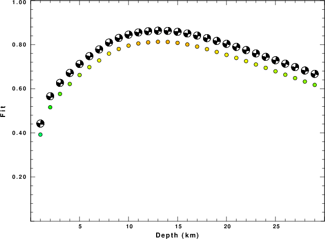
The best fit as a function of depth is given in the following figure:
|
|
Figure 2. Depth sensitivity for waveform mechanism
|
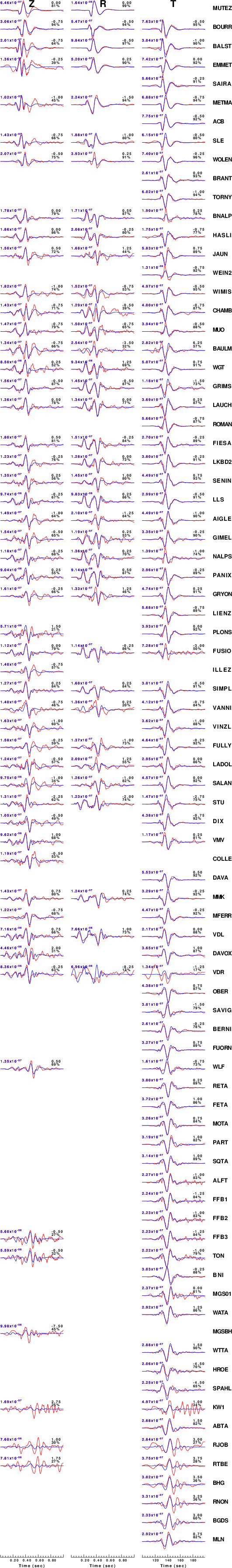
The comparison of the observed and predicted waveforms is given in the next figure. The red traces are the observed and the blue are the predicted.
Each observed-predicted component is plotted to the same scale and peak amplitudes are indicated by the numbers to the left of each trace. A pair of numbers is given in black at the right of each predicted traces. The upper number it the time shift required for maximum correlation between the observed and predicted traces. This time shift is required because the synthetics are not computed at exactly the same distance as the observed and because the velocity model used in the predictions may not be perfect.
A positive time shift indicates that the prediction is too fast and should be delayed to match the observed trace (shift to the right in this figure). A negative value indicates that the prediction is too slow. The lower number gives the percentage of variance reduction to characterize the individual goodness of fit (100% indicates a perfect fit).
The bandpass filter used in the processing and for the display was
cut o DIST/3.3 -30 o DIST/3.3 +70
rtr
taper w 0.1
hp c 0.03 n 3
lp c 0.06 n 3
|
|
Figure 3. Waveform comparison for selected depth
|
|
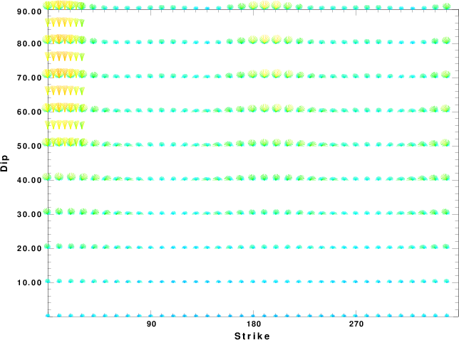
|
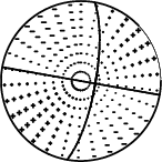
Focal mechanism sensitivity at the preferred depth. The red color indicates a very good fit to thewavefroms.
Each solution is plotted as a vector at a given value of strike and dip with the angle of the vector representing the rake angle, measured, with respect to the upward vertical (N) in the figure.
|
A check on the assumed source location is possible by looking at the time shifts between the observed and predicted traces. The time shifts for waveform matching arise for several reasons:
- The origin time and epicentral distance are incorrect
- The velocity model used for the inversion is incorrect
- The velocity model used to define the P-arrival time is not the
same as the velocity model used for the waveform inversion
(assuming that the initial trace alignment is based on the
P arrival time)
Assuming only a mislocation, the time shifts are fit to a functional form:
Time_shift = A + B cos Azimuth + C Sin Azimuth
The time shifts for this inversion lead to the next figure:
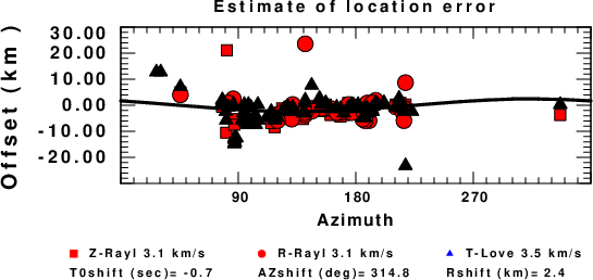
The derived shift in origin time and epicentral coordinates are given at the bottom of the figure.
Discussion
Acknowledgements
Thanks also to the many seismic network operators whose dedication make this effort possible: University of Nevada Reno, University of Alaska, University of Washington, Oregon State University, University of Utah, Montana Bureas of Mines, UC Berkely, Caltech, UC San Diego, Saint Louis University, University of Memphis, Lamont Doherty Earth Observatory, the Iris stations and the Transportable Array of EarthScope.
Velocity Model
The WUS.model used for the waveform synthetic seismograms and for the surface wave eigenfunctions and dispersion is as follows:
MODEL.01
Model after     8 iterations
ISOTROPIC
KGS
FLAT EARTH
1-D
CONSTANT VELOCITY
LINE08
LINE09
LINE10
LINE11
      H(KM)   VP(KM/S)   VS(KM/S) RHO(GM/CC)         QP         QS       ETAP       ETAS      FREFP      FREFS
     1.9000     3.4065     2.0089     2.2150  0.302E-02  0.679E-02   0.00       0.00       1.00       1.00
     6.1000     5.5445     3.2953     2.6089  0.349E-02  0.784E-02   0.00       0.00       1.00       1.00
    13.0000     6.2708     3.7396     2.7812  0.212E-02  0.476E-02   0.00       0.00       1.00       1.00
    19.0000     6.4075     3.7680     2.8223  0.111E-02  0.249E-02   0.00       0.00       1.00       1.00
     0.0000     7.9000     4.6200     3.2760  0.164E-10  0.370E-10   0.00       0.00       1.00       1.00
Quality Control
Here we tabulate the reasons for not using certain digital data sets
The following stations did not have a valid response files:
Last Changed Sun Sep 11 13:07:18 CDT 2022