Location
Location ANSS
2020/05/08 12:47:44 41.83 2.66 5.0 3.7 Catulunya, Spain
Focal Mechanism
 USGS/SLU Moment Tensor Solution
 ENS  2020/05/08 12:47:44:0  41.83    2.66   5.0 3.7 Catulunya, Spain

 Stations used:
   CA.ARBS CA.CAVN CA.CBEU CA.CBRU CA.CBUD CA.CCAS CA.CEST
   CA.CGAR CA.CLLI CA.CMAS CA.CORG CA.CORI CA.CPAL CA.CSOR
   CA.CTRE CA.EBR IU.PAB LC.CANF

 Filtering commands used:
   cut o DIST/3.3 -40 o DIST/3.3 +50
   rtr
   taper w 0.1
   hp c 0.03 n 3
   lp c 0.10 n 3

 Best Fitting Double Couple
  Mo = 1.16e+21 dyne-cm
  Mw = 3.31
  Z  = 12 km
  Plane   Strike  Dip  Rake
   NP1        5    55   -70
   NP2      153    40   -116
  Principal Axes:
   Axis    Value   Plunge  Azimuth
    T   1.16e+21      8      81
    N   0.00e+00     16     173
    P  -1.16e+21     72     326

 Moment Tensor: (dyne-cm)
    Component   Value
       Mxx    -4.87e+19
       Mxy     2.31e+20
       Mxz    -2.60e+20
       Myy     1.07e+21
       Myz     3.52e+20
       Mzz    -1.03e+21


                     ----------####
                 #---------------######
              ###-----------------########
             ###-------------------########
           ####--------------------##########
          #####---------------------##########
         #####----------------------###########
        ######---------   -----------###########
        ######--------- P -----------#########
       #######---------   -----------######### T
       ########----------------------#########
       ########----------------------############
       #########---------------------############
        ########--------------------############
        #########-------------------############
         #########-----------------############
          ##########---------------###########
           ##########-------------###########
             ###########---------##########
              ############------##########
                 ######################
                     #######-------


 Global CMT Convention Moment Tensor:
      R          T          P
 -1.03e+21  -2.60e+20  -3.52e+20
 -2.60e+20  -4.87e+19  -2.31e+20
 -3.52e+20  -2.31e+20   1.07e+21


Details of the solution is found at

http://www.eas.slu.edu/eqc/eqc_mt/MECH.NA/20200508124744/index.html
|
Preferred Solution
The preferred solution from an analysis of the surface-wave spectral amplitude radiation pattern, waveform inversion and first motion observations is
      STK = 5
      DIP = 55
     RAKE = -70
       MW = 3.31
       HS = 12.0
The NDK file is 20200508124744.ndk
The waveform inversion is preferred.
Moment Tensor Comparison
The following compares this source inversion to others
| SLU |
IGN |
 USGS/SLU Moment Tensor Solution
 ENS  2020/05/08 12:47:44:0  41.83    2.66   5.0 3.7 Catulunya, Spain

 Stations used:
   CA.ARBS CA.CAVN CA.CBEU CA.CBRU CA.CBUD CA.CCAS CA.CEST
   CA.CGAR CA.CLLI CA.CMAS CA.CORG CA.CORI CA.CPAL CA.CSOR
   CA.CTRE CA.EBR IU.PAB LC.CANF

 Filtering commands used:
   cut o DIST/3.3 -40 o DIST/3.3 +50
   rtr
   taper w 0.1
   hp c 0.03 n 3
   lp c 0.10 n 3

 Best Fitting Double Couple
  Mo = 1.16e+21 dyne-cm
  Mw = 3.31
  Z  = 12 km
  Plane   Strike  Dip  Rake
   NP1        5    55   -70
   NP2      153    40   -116
  Principal Axes:
   Axis    Value   Plunge  Azimuth
    T   1.16e+21      8      81
    N   0.00e+00     16     173
    P  -1.16e+21     72     326

 Moment Tensor: (dyne-cm)
    Component   Value
       Mxx    -4.87e+19
       Mxy     2.31e+20
       Mxz    -2.60e+20
       Myy     1.07e+21
       Myz     3.52e+20
       Mzz    -1.03e+21


                     ----------####
                 #---------------######
              ###-----------------########
             ###-------------------########
           ####--------------------##########
          #####---------------------##########
         #####----------------------###########
        ######---------   -----------###########
        ######--------- P -----------#########
       #######---------   -----------######### T
       ########----------------------#########
       ########----------------------############
       #########---------------------############
        ########--------------------############
        #########-------------------############
         #########-----------------############
          ##########---------------###########
           ##########-------------###########
             ###########---------##########
              ############------##########
                 ######################
                     #######-------


 Global CMT Convention Moment Tensor:
      R          T          P
 -1.03e+21  -2.60e+20  -3.52e+20
 -2.60e+20  -4.87e+19  -2.31e+20
 -3.52e+20  -2.31e+20   1.07e+21


Details of the solution is found at

http://www.eas.slu.edu/eqc/eqc_mt/MECH.NA/20200508124744/index.html
|
Evid        Date      Time (UTC) Latitude Longitude Prof. centroid Mw Location
es2020jaxat 05/08/2020 12:47:44  41.8324  2.6683      5        3.5 S  SANTA COLOMA DE FARNERS.GI

Components of the deviant TMS (null isotropic part) - (10 ^ 20 dyne-cm)
M0 mzz mxx myy mxz myz mxy
22.00E20 -9,806 9,874 -0.068 -16,582 3,796 9,833

TMS decomposition Double even percentage: 92 Dipole percentage: 8

Double pair: Plane A  Double pair: Plane B
Azimuth: 88           Azimuth: 333
Dip: 75               Dip: 32
Glide: -119           Slip: -29

Fit quality
Variance reduction [0-100]: 67
Automatic TMS calculation detail

Available images
 Focal Mechanism
|
Magnitudes
mLg Magnitude
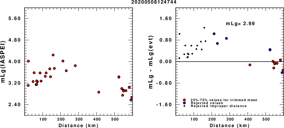
(a) mLg computed using the IASPEI formula; (b) mLg residuals ; the values used for the trimmed mean are indicated.
ML Magnitude
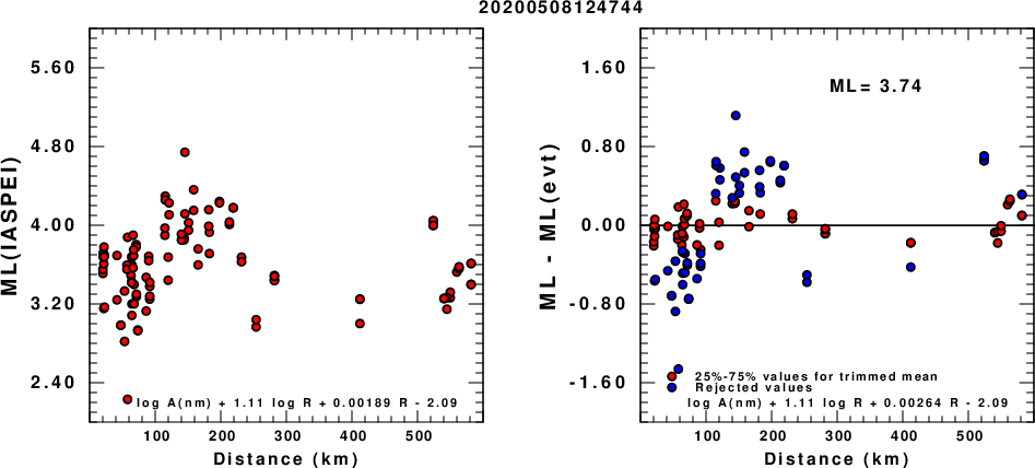
(a) ML computed using the IASPEI formula for Horizontal components; (b) ML residuals computed using a modified IASPEI formula that accounts for path specific attenuation; the values used for the trimmed mean are indicated. The ML relation used for each figure is given at the bottom of each plot.
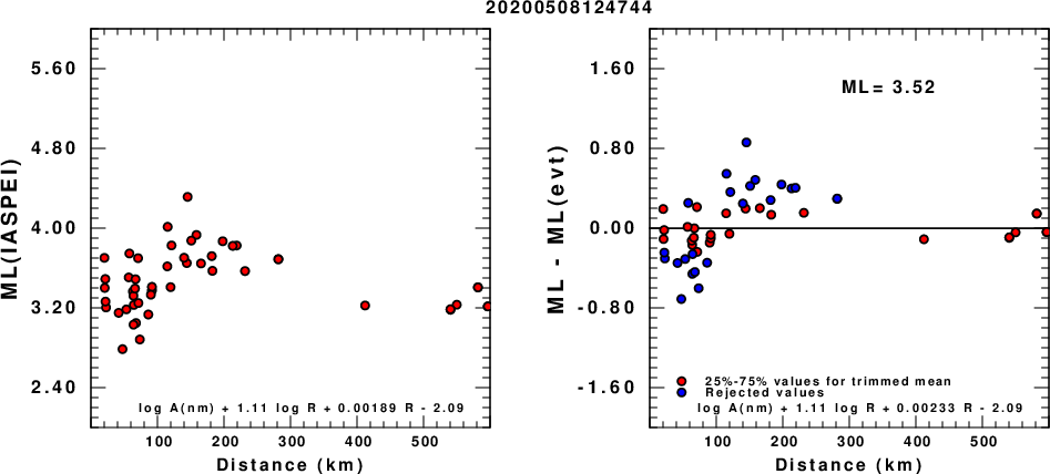
(a) ML computed using the IASPEI formula for Vertical components (research); (b) ML residuals computed using a modified IASPEI formula that accounts for path specific attenuation; the values used for the trimmed mean are indicated. The ML relation used for each figure is given at the bottom of each plot.
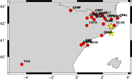
Context
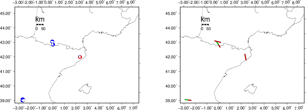
The next figure presents the focal mechanism for this earthquake (red) in the context of other events (blue) in the SLU Moment Tensor Catalog which are within ± 0.5 degrees of the new event. This comparison is shown in the left panel of the figure. The right panel shows the inferred direction of maximum compressive stress and the type of faulting (green is strike-slip, red is normal, blue is thrust; oblique is shown by a combination of colors).
Waveform Inversion using wvfgrd96
The focal mechanism was determined using broadband seismic waveforms. The location of the event and the
and stations used for the waveform inversion are shown in the next figure.
|
|
Location of broadband stations used for waveform inversion
|
The program wvfgrd96 was used with good traces observed at short distance to determine the focal mechanism, depth and seismic moment. This technique requires a high quality signal and well determined velocity model for the Green functions. To the extent that these are the quality data, this type of mechanism should be preferred over the radiation pattern technique which requires the separate step of defining the pressure and tension quadrants and the correct strike.
The observed and predicted traces are filtered using the following gsac commands:
cut o DIST/3.3 -40 o DIST/3.3 +50
rtr
taper w 0.1
hp c 0.03 n 3
lp c 0.10 n 3
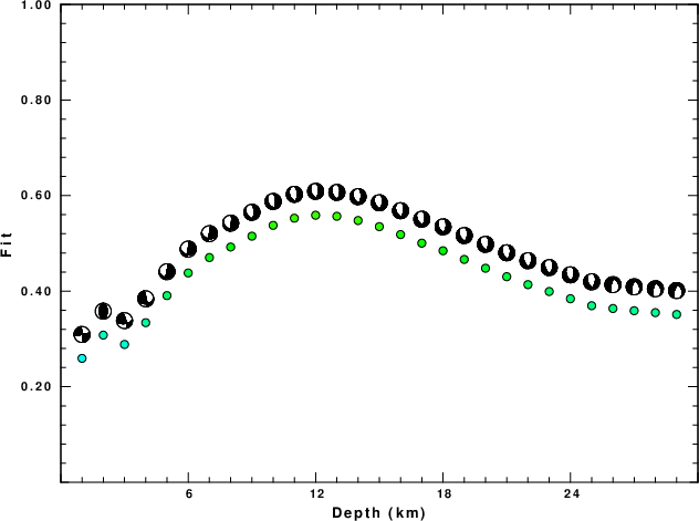
The results of this grid search from 0.5 to 19 km depth are as follow:
           DEPTH  STK   DIP  RAKE   MW    FIT
WVFGRD96    1.0   260    90    -5   2.90 0.2594
WVFGRD96    2.0   180    45    90   3.03 0.3081
WVFGRD96    3.0    85    55    20   3.12 0.2885
WVFGRD96    4.0    85    35    10   3.14 0.3341
WVFGRD96    5.0    10    90   -65   3.13 0.3908
WVFGRD96    6.0    10    90   -60   3.14 0.4381
WVFGRD96    7.0    10    90   -55   3.16 0.4703
WVFGRD96    8.0     5    80   -65   3.23 0.4924
WVFGRD96    9.0     0    65   -70   3.26 0.5151
WVFGRD96   10.0     0    60   -70   3.28 0.5377
WVFGRD96   11.0     0    55   -75   3.30 0.5527
WVFGRD96   12.0     5    55   -70   3.31 0.5589
WVFGRD96   13.0     5    55   -70   3.32 0.5567
WVFGRD96   14.0     5    55   -70   3.33 0.5478
WVFGRD96   15.0    10    55   -65   3.34 0.5350
WVFGRD96   16.0    10    55   -65   3.35 0.5184
WVFGRD96   17.0    10    55   -60   3.35 0.5005
WVFGRD96   18.0    10    55   -60   3.36 0.4846
WVFGRD96   19.0    10    55   -60   3.37 0.4664
WVFGRD96   20.0    10    55   -60   3.37 0.4480
WVFGRD96   21.0    10    50   -65   3.38 0.4303
WVFGRD96   22.0    15    50   -60   3.39 0.4137
WVFGRD96   23.0    15    50   -60   3.39 0.3993
WVFGRD96   24.0    15    50   -60   3.40 0.3842
WVFGRD96   25.0    15    50   -60   3.40 0.3696
WVFGRD96   26.0   195    70   -65   3.41 0.3637
WVFGRD96   27.0   195    65   -65   3.42 0.3591
WVFGRD96   28.0   195    65   -65   3.42 0.3551
WVFGRD96   29.0   200    65   -65   3.43 0.3513
The best solution is
WVFGRD96 12.0 5 55 -70 3.31 0.5589
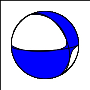
The mechanism correspond to the best fit is
|
|
Figure 1. Waveform inversion focal mechanism
|
The best fit as a function of depth is given in the following figure:
|
|
Figure 2. Depth sensitivity for waveform mechanism
|
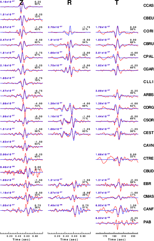
The comparison of the observed and predicted waveforms is given in the next figure. The red traces are the observed and the blue are the predicted.
Each observed-predicted component is plotted to the same scale and peak amplitudes are indicated by the numbers to the left of each trace. A pair of numbers is given in black at the right of each predicted traces. The upper number it the time shift required for maximum correlation between the observed and predicted traces. This time shift is required because the synthetics are not computed at exactly the same distance as the observed and because the velocity model used in the predictions may not be perfect.
A positive time shift indicates that the prediction is too fast and should be delayed to match the observed trace (shift to the right in this figure). A negative value indicates that the prediction is too slow. The lower number gives the percentage of variance reduction to characterize the individual goodness of fit (100% indicates a perfect fit).
The bandpass filter used in the processing and for the display was
cut o DIST/3.3 -40 o DIST/3.3 +50
rtr
taper w 0.1
hp c 0.03 n 3
lp c 0.10 n 3
|
|
Figure 3. Waveform comparison for selected depth. Red: observed; Blue - predicted. The time shift with respect to the model prediction is indicated. The percent of fit is also indicated.
|
|
|
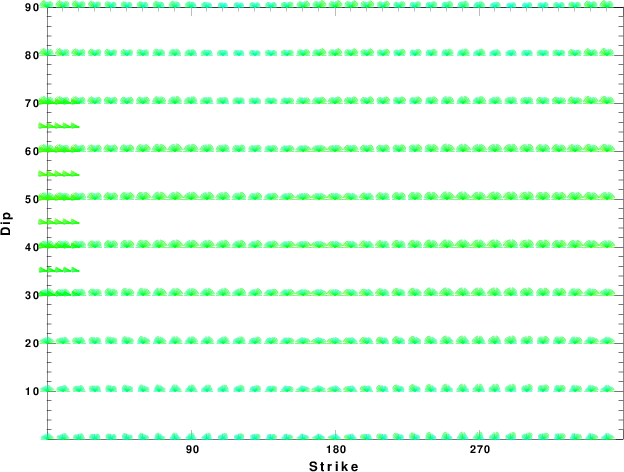
Focal mechanism sensitivity at the preferred depth. The red color indicates a very good fit to thewavefroms.
Each solution is plotted as a vector at a given value of strike and dip with the angle of the vector representing the rake angle, measured, with respect to the upward vertical (N) in the figure.
|
A check on the assumed source location is possible by looking at the time shifts between the observed and predicted traces. The time shifts for waveform matching arise for several reasons:
- The origin time and epicentral distance are incorrect
- The velocity model used for the inversion is incorrect
- The velocity model used to define the P-arrival time is not the
same as the velocity model used for the waveform inversion
(assuming that the initial trace alignment is based on the
P arrival time)
Assuming only a mislocation, the time shifts are fit to a functional form:
Time_shift = A + B cos Azimuth + C Sin Azimuth
The time shifts for this inversion lead to the next figure:
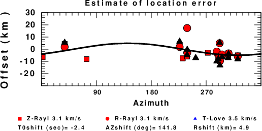
The derived shift in origin time and epicentral coordinates are given at the bottom of the figure.
Discussion
Acknowledgements
Thanks also to the many seismic network operators whose dedication make this effort possible: University of Nevada Reno, University of Alaska, University of Washington, Oregon State University, University of Utah, Montana Bureau of Mines, UC Berkely, Caltech, UC San Diego, Saint Louis University, University of Memphis, Lamont Doherty Earth Observatory, the Oklahoma Geological Survey, TexNet, the Iris stations, the Transportable Array of EarthScope and other networks.
Velocity Model
The WUS.model used for the waveform synthetic seismograms and for the surface wave eigenfunctions and dispersion is as follows:
MODEL.01
Model after     8 iterations
ISOTROPIC
KGS
FLAT EARTH
1-D
CONSTANT VELOCITY
LINE08
LINE09
LINE10
LINE11
      H(KM)   VP(KM/S)   VS(KM/S) RHO(GM/CC)         QP         QS       ETAP       ETAS      FREFP      FREFS
     1.9000     3.4065     2.0089     2.2150  0.302E-02  0.679E-02   0.00       0.00       1.00       1.00
     6.1000     5.5445     3.2953     2.6089  0.349E-02  0.784E-02   0.00       0.00       1.00       1.00
    13.0000     6.2708     3.7396     2.7812  0.212E-02  0.476E-02   0.00       0.00       1.00       1.00
    19.0000     6.4075     3.7680     2.8223  0.111E-02  0.249E-02   0.00       0.00       1.00       1.00
     0.0000     7.9000     4.6200     3.2760  0.164E-10  0.370E-10   0.00       0.00       1.00       1.00
Quality Control
Here we tabulate the reasons for not using certain digital data sets
The following stations did not have a valid response files:
Last Changed Wed May 13 14:27:35 CDT 2020