Location
Location ANSS
2019/09/21 14:04:25 41.36 19.40 10.0 5.7 Albania
Focal Mechanism
 USGS/SLU Moment Tensor Solution
 ENS  2019/09/21 14:04:25:2  41.36   19.40  10.0 5.7 Albania

 Stations used:
   AC.KBN AC.VLO BS.ELND BS.PLVB CL.AGRP CL.MALA CL.MG00
   CL.MG02 CL.MG05 CL.PSAM CL.TRIZ CR.ZAG HA.ATAL HA.ATHU
   HA.AXAR HA.KALE HA.KARY HA.LOUT HA.MAGU HA.MAKR HA.VILL
   HL.ATH HL.EVR HL.ITM HL.JAN HL.KEK HL.KYMI HL.KZN HL.LIA
   HL.LKR HL.NEO HL.PENT HL.PLG HL.PRK HL.PTL HL.RDO HL.SKY
   HL.SMTH HL.TETR HL.VLS HL.VLY HP.AMPL HP.AMT HP.ANX HP.DRO
   HP.EFP HP.FSK HP.GUR HP.LTK HP.PRMD HP.PVO HP.SERG HT.AGG
   HT.ALN HT.EVGI HT.IGT HT.KAVA HT.KNT HT.LIT HT.LKD2 HT.OUR
   HT.PAIG HT.SIGR HT.SOH HT.SRS HT.THAS HT.THE HU.BSZH HU.BUD
   HU.CSKK HU.EGYH HU.KOVH HU.TIH KO.GADA MN.KEK MN.KLV MN.PDG
   MN.THL MN.TRI OE.SOKA RO.BAIL RO.BANR RO.BZS RO.CJR RO.DEV
   RO.DRGR RO.GZR RO.HERR RO.HUMR RO.LOT RO.PUNG RO.SIRR
   RO.SULR RO.VLAD RO.VOIR SJ.BBLS SJ.FRGS

 Filtering commands used:
   cut o DIST/3.3 -30 o DIST/3.3 +70
   rtr
   taper w 0.1
   hp c 0.02 n 3
   lp c 0.05 n 3

 Best Fitting Double Couple
  Mo = 2.75e+24 dyne-cm
  Mw = 5.56
  Z  = 22 km
  Plane   Strike  Dip  Rake
   NP1      149    65    88
   NP2      335    25    95
  Principal Axes:
   Axis    Value   Plunge  Azimuth
    T   2.75e+24     70      55
    N   0.00e+00      2     150
    P  -2.75e+24     20     241

 Moment Tensor: (dyne-cm)
    Component   Value
       Mxx    -4.53e+23
       Mxy    -8.70e+23
       Mxz     9.43e+23
       Myy    -1.65e+24
       Myz     1.51e+24
       Mzz     2.10e+24


                     --------------
                 ##############--------
              ---##################-------
             ----####################------
           ------######################------
          -------#######################------
         ---------#######################------
        ----------########################------
        -----------############   #########-----
       -------------########### T ##########-----
       -------------###########   ##########-----
       --------------#######################-----
       ---------------######################-----
        ---------------#####################----
        ----   ----------###################----
         --- P -----------##################---
          --   -------------###############---
           ------------------#############---
             ------------------##########--
              --------------------######--
                 ----------------------
                     --------------


 Global CMT Convention Moment Tensor:
      R          T          P
  2.10e+24   9.43e+23  -1.51e+24
  9.43e+23  -4.53e+23   8.70e+23
 -1.51e+24   8.70e+23  -1.65e+24


Details of the solution is found at

http://www.eas.slu.edu/eqc/eqc_mt/MECH.NA/20190921140425/index.html
|
Preferred Solution
The preferred solution from an analysis of the surface-wave spectral amplitude radiation pattern, waveform inversion and first motion observations is
      STK = 335
      DIP = 25
     RAKE = 95
       MW = 5.56
       HS = 22.0
The NDK file is 20190921140425.ndk
The waveform inversion is preferred.
Moment Tensor Comparison
The following compares this source inversion to others
| SLU |
USGSW |
 USGS/SLU Moment Tensor Solution
 ENS  2019/09/21 14:04:25:2  41.36   19.40  10.0 5.7 Albania

 Stations used:
   AC.KBN AC.VLO BS.ELND BS.PLVB CL.AGRP CL.MALA CL.MG00
   CL.MG02 CL.MG05 CL.PSAM CL.TRIZ CR.ZAG HA.ATAL HA.ATHU
   HA.AXAR HA.KALE HA.KARY HA.LOUT HA.MAGU HA.MAKR HA.VILL
   HL.ATH HL.EVR HL.ITM HL.JAN HL.KEK HL.KYMI HL.KZN HL.LIA
   HL.LKR HL.NEO HL.PENT HL.PLG HL.PRK HL.PTL HL.RDO HL.SKY
   HL.SMTH HL.TETR HL.VLS HL.VLY HP.AMPL HP.AMT HP.ANX HP.DRO
   HP.EFP HP.FSK HP.GUR HP.LTK HP.PRMD HP.PVO HP.SERG HT.AGG
   HT.ALN HT.EVGI HT.IGT HT.KAVA HT.KNT HT.LIT HT.LKD2 HT.OUR
   HT.PAIG HT.SIGR HT.SOH HT.SRS HT.THAS HT.THE HU.BSZH HU.BUD
   HU.CSKK HU.EGYH HU.KOVH HU.TIH KO.GADA MN.KEK MN.KLV MN.PDG
   MN.THL MN.TRI OE.SOKA RO.BAIL RO.BANR RO.BZS RO.CJR RO.DEV
   RO.DRGR RO.GZR RO.HERR RO.HUMR RO.LOT RO.PUNG RO.SIRR
   RO.SULR RO.VLAD RO.VOIR SJ.BBLS SJ.FRGS

 Filtering commands used:
   cut o DIST/3.3 -30 o DIST/3.3 +70
   rtr
   taper w 0.1
   hp c 0.02 n 3
   lp c 0.05 n 3

 Best Fitting Double Couple
  Mo = 2.75e+24 dyne-cm
  Mw = 5.56
  Z  = 22 km
  Plane   Strike  Dip  Rake
   NP1      149    65    88
   NP2      335    25    95
  Principal Axes:
   Axis    Value   Plunge  Azimuth
    T   2.75e+24     70      55
    N   0.00e+00      2     150
    P  -2.75e+24     20     241

 Moment Tensor: (dyne-cm)
    Component   Value
       Mxx    -4.53e+23
       Mxy    -8.70e+23
       Mxz     9.43e+23
       Myy    -1.65e+24
       Myz     1.51e+24
       Mzz     2.10e+24


                     --------------
                 ##############--------
              ---##################-------
             ----####################------
           ------######################------
          -------#######################------
         ---------#######################------
        ----------########################------
        -----------############   #########-----
       -------------########### T ##########-----
       -------------###########   ##########-----
       --------------#######################-----
       ---------------######################-----
        ---------------#####################----
        ----   ----------###################----
         --- P -----------##################---
          --   -------------###############---
           ------------------#############---
             ------------------##########--
              --------------------######--
                 ----------------------
                     --------------


 Global CMT Convention Moment Tensor:
      R          T          P
  2.10e+24   9.43e+23  -1.51e+24
  9.43e+23  -4.53e+23   8.70e+23
 -1.51e+24   8.70e+23  -1.65e+24


Details of the solution is found at

http://www.eas.slu.edu/eqc/eqc_mt/MECH.NA/20190921140425/index.html
|
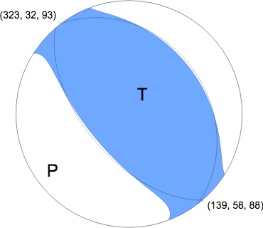
W-phase Moment Tensor (Mww)
Moment 3.691e+17 N-m
Magnitude 5.64 Mww
Depth 17.5 km
Percent DC 79%
Half Duration 1.61 s
Catalog US
Data Source US 1
Contributor US 1

Nodal Planes
Plane Strike Dip Rake
NP1 323 32 93
NP2 139 58 88

Principal Axes
Axis Value Plunge Azimuth
T 3.476e+17 N-m 76 44
N 0.397e+17 N-m 1 140
P -3.873e+17 N-m 13 231
|
Magnitudes
mLg Magnitude
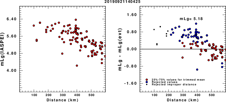
(a) mLg computed using the IASPEI formula; (b) mLg residuals ; the values used for the trimmed mean are indicated.
ML Magnitude
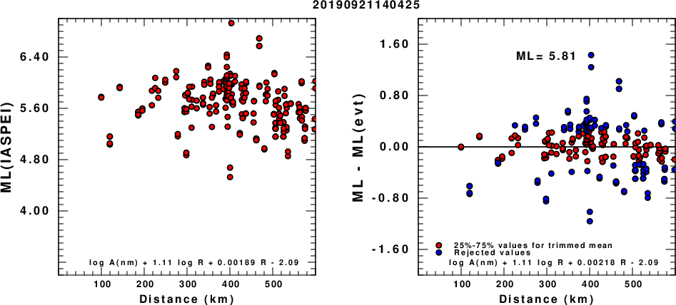
(a) ML computed using the IASPEI formula for Horizontal components; (b) ML residuals computed using a modified IASPEI formula that accounts for path specific attenuation; the values used for the trimmed mean are indicated. The ML relation used for each figure is given at the bottom of each plot.
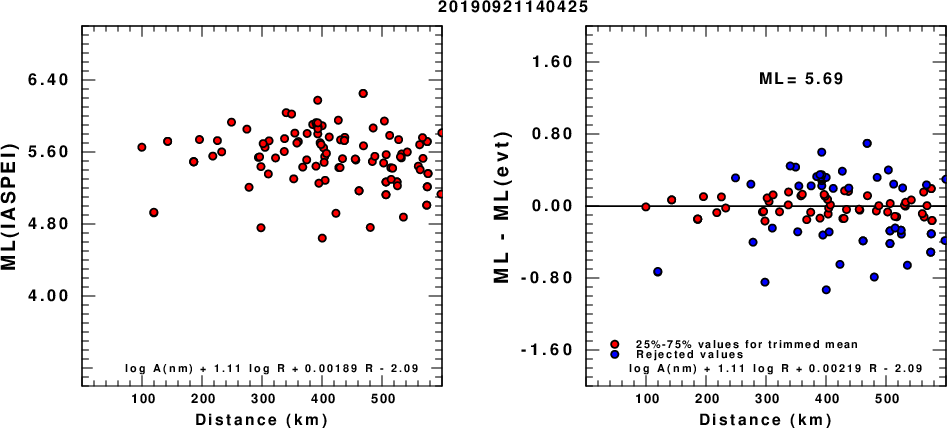
(a) ML computed using the IASPEI formula for Vertical components (research); (b) ML residuals computed using a modified IASPEI formula that accounts for path specific attenuation; the values used for the trimmed mean are indicated. The ML relation used for each figure is given at the bottom of each plot.
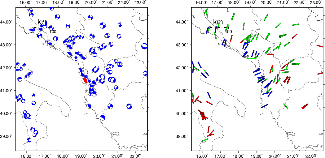
Context
The next figure presents the focal mechanism for this earthquake (red) in the context of other events (blue) in the SLU Moment Tensor Catalog which are within ± 0.5 degrees of the new event. This comparison is shown in the left panel of the figure. The right panel shows the inferred direction of maximum compressive stress and the type of faulting (green is strike-slip, red is normal, blue is thrust; oblique is shown by a combination of colors).
Waveform Inversion
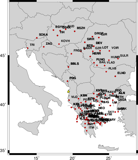
The focal mechanism was determined using broadband seismic waveforms. The location of the event and the
and stations used for the waveform inversion are shown in the next figure.
|
|
Location of broadband stations used for waveform inversion
|
The program wvfgrd96 was used with good traces observed at short distance to determine the focal mechanism, depth and seismic moment. This technique requires a high quality signal and well determined velocity model for the Green functions. To the extent that these are the quality data, this type of mechanism should be preferred over the radiation pattern technique which requires the separate step of defining the pressure and tension quadrants and the correct strike.
The observed and predicted traces are filtered using the following gsac commands:
cut o DIST/3.3 -30 o DIST/3.3 +70
rtr
taper w 0.1
hp c 0.02 n 3
lp c 0.05 n 3
The results of this grid search from 0.5 to 19 km depth are as follow:
           DEPTH  STK   DIP  RAKE   MW    FIT
WVFGRD96    1.0   260    45   -70   5.12 0.1716
WVFGRD96    2.0   260    45   -70   5.20 0.2019
WVFGRD96    3.0   260    45   -70   5.27 0.2200
WVFGRD96    4.0   275    50   -45   5.29 0.2207
WVFGRD96    5.0   285    55   -25   5.29 0.2214
WVFGRD96    6.0   285    55   -25   5.31 0.2226
WVFGRD96    7.0   285    55   -20   5.32 0.2251
WVFGRD96    8.0   285    50   -20   5.36 0.2285
WVFGRD96    9.0   290    45     0   5.37 0.2303
WVFGRD96   10.0   335    25    90   5.49 0.2458
WVFGRD96   11.0   155    65    90   5.51 0.2679
WVFGRD96   12.0   155    65    90   5.51 0.2865
WVFGRD96   13.0   155    65    90   5.52 0.3018
WVFGRD96   14.0   340    30    95   5.52 0.3144
WVFGRD96   15.0   155    60    90   5.53 0.3248
WVFGRD96   16.0   155    60    90   5.53 0.3329
WVFGRD96   17.0   155    60    90   5.53 0.3389
WVFGRD96   18.0   150    60    85   5.54 0.3435
WVFGRD96   19.0   155    60    90   5.54 0.3466
WVFGRD96   20.0   150    65    85   5.55 0.3486
WVFGRD96   21.0   340    30    95   5.56 0.3518
WVFGRD96   22.0   335    25    95   5.56 0.3521
WVFGRD96   23.0   150    65    85   5.56 0.3518
WVFGRD96   24.0   150    65    90   5.57 0.3507
WVFGRD96   25.0   150    65    90   5.57 0.3491
WVFGRD96   26.0   150    65    90   5.57 0.3469
WVFGRD96   27.0   325    25    85   5.58 0.3444
WVFGRD96   28.0   325    25    85   5.58 0.3413
WVFGRD96   29.0   320    25    80   5.58 0.3377
The best solution is
WVFGRD96 22.0 335 25 95 5.56 0.3521
The mechanism correspond to the best fit is
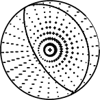
|
|
Figure 1. Waveform inversion focal mechanism
|
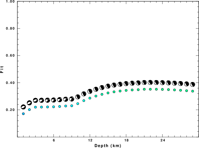
The best fit as a function of depth is given in the following figure:
|
|
Figure 2. Depth sensitivity for waveform mechanism
|
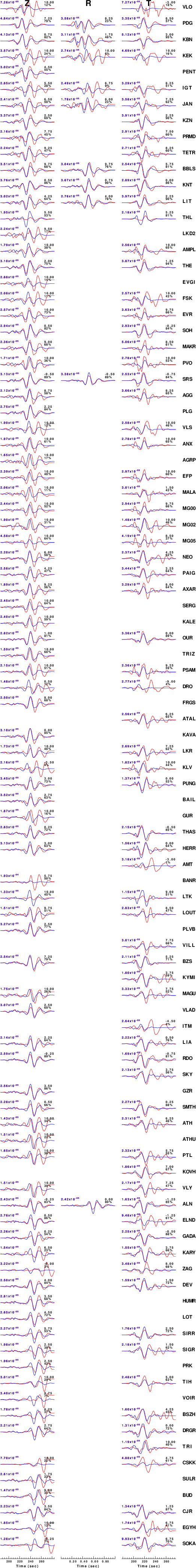
The comparison of the observed and predicted waveforms is given in the next figure. The red traces are the observed and the blue are the predicted.
Each observed-predicted component is plotted to the same scale and peak amplitudes are indicated by the numbers to the left of each trace. A pair of numbers is given in black at the right of each predicted traces. The upper number it the time shift required for maximum correlation between the observed and predicted traces. This time shift is required because the synthetics are not computed at exactly the same distance as the observed and because the velocity model used in the predictions may not be perfect.
A positive time shift indicates that the prediction is too fast and should be delayed to match the observed trace (shift to the right in this figure). A negative value indicates that the prediction is too slow. The lower number gives the percentage of variance reduction to characterize the individual goodness of fit (100% indicates a perfect fit).
The bandpass filter used in the processing and for the display was
cut o DIST/3.3 -30 o DIST/3.3 +70
rtr
taper w 0.1
hp c 0.02 n 3
lp c 0.05 n 3
|
|
Figure 3. Waveform comparison for selected depth
|
|
|
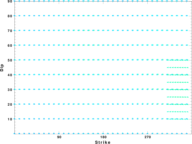
Focal mechanism sensitivity at the preferred depth. The red color indicates a very good fit to thewavefroms.
Each solution is plotted as a vector at a given value of strike and dip with the angle of the vector representing the rake angle, measured, with respect to the upward vertical (N) in the figure.
|
A check on the assumed source location is possible by looking at the time shifts between the observed and predicted traces. The time shifts for waveform matching arise for several reasons:
- The origin time and epicentral distance are incorrect
- The velocity model used for the inversion is incorrect
- The velocity model used to define the P-arrival time is not the
same as the velocity model used for the waveform inversion
(assuming that the initial trace alignment is based on the
P arrival time)
Assuming only a mislocation, the time shifts are fit to a functional form:
Time_shift = A + B cos Azimuth + C Sin Azimuth
The time shifts for this inversion lead to the next figure:
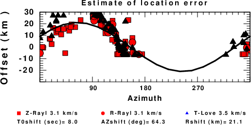
The derived shift in origin time and epicentral coordinates are given at the bottom of the figure.
Discussion
Acknowledgements
Thanks also to the many seismic network operators whose dedication make this effort possible: University of Nevada Reno, University of Alaska, University of Washington, Oregon State University, University of Utah, Montana Bureas of Mines, UC Berkely, Caltech, UC San Diego, Saint Louis University, University of Memphis, Lamont Doherty Earth Observatory, the Iris stations and the Transportable Array of EarthScope.
Velocity Model
The WUS.model used for the waveform synthetic seismograms and for the surface wave eigenfunctions and dispersion is as follows:
MODEL.01
Model after     8 iterations
ISOTROPIC
KGS
FLAT EARTH
1-D
CONSTANT VELOCITY
LINE08
LINE09
LINE10
LINE11
      H(KM)   VP(KM/S)   VS(KM/S) RHO(GM/CC)         QP         QS       ETAP       ETAS      FREFP      FREFS
     1.9000     3.4065     2.0089     2.2150  0.302E-02  0.679E-02   0.00       0.00       1.00       1.00
     6.1000     5.5445     3.2953     2.6089  0.349E-02  0.784E-02   0.00       0.00       1.00       1.00
    13.0000     6.2708     3.7396     2.7812  0.212E-02  0.476E-02   0.00       0.00       1.00       1.00
    19.0000     6.4075     3.7680     2.8223  0.111E-02  0.249E-02   0.00       0.00       1.00       1.00
     0.0000     7.9000     4.6200     3.2760  0.164E-10  0.370E-10   0.00       0.00       1.00       1.00
Quality Control
Here we tabulate the reasons for not using certain digital data sets
The following stations did not have a valid response files:
Last Changed Sun Sep 22 11:03:38 CDT 2019