Location
2016/09/23 23:11:20 45.76 26.63 94 5.6 Romania
Arrival Times (from USGS)
Arrival time list
Felt Map
USGS Felt map for this earthquake
USGS Felt reports archive
Focal Mechanism
 USGS/SLU Moment Tensor Solution
 ENS  2016/09/23 23:11:20:0  45.76   26.63  94.0 5.6 Romania

 Stations used:
   GE.PSZ GE.TIRR HT.ALN HT.KNT HU.BSZH HU.BUD HU.KOVH HU.LTVH
   HU.TRPA KO.ARMT KO.ISK MN.DIVS MN.PDG MN.VTS SJ.FRGS

 Filtering commands used:
   cut a -30 a 210
   rtr
   taper w 0.1
   hp c 0.015 n 3
   lp c 0.04 n 3

 Best Fitting Double Couple
  Mo = 3.16e+24 dyne-cm
  Mw = 5.60
  Z  = 92 km
  Plane   Strike  Dip  Rake
   NP1      310    59   106
   NP2      100    35    65
  Principal Axes:
   Axis    Value   Plunge  Azimuth
    T   3.16e+24     71     258
    N   0.00e+00     14     121
    P  -3.16e+24     12      28

 Moment Tensor: (dyne-cm)
    Component   Value
       Mxx    -2.35e+24
       Mxy    -1.18e+24
       Mxz    -7.75e+23
       Myy    -3.43e+23
       Myz    -1.25e+24
       Mzz     2.69e+24


                     --------------
                 ------------------   -
              --------------------- P ----
             ----------------------   -----
           ############----------------------
          #################-------------------
         #####################-----------------
        #########################---------------
        ###########################-------------
       -#############################------------
       -##############   #############-----------
       --############# T ###############---------
       ---############   ################--------
        ---###############################------
        -----##############################---##
         ------############################--##
          -------#########################--##
           ----------##################-----#
             ------------------------------
              ----------------------------
                 ----------------------
                     --------------


 Global CMT Convention Moment Tensor:
      R          T          P
  2.69e+24  -7.75e+23   1.25e+24
 -7.75e+23  -2.35e+24   1.18e+24
  1.25e+24   1.18e+24  -3.43e+23


Details of the solution is found at

http://www.eas.slu.edu/eqc/eqc_mt/MECH.EU/20160923231120/index.html
|
Preferred Solution
The preferred solution from an analysis of the surface-wave spectral amplitude radiation pattern, waveform inversion and first motion observations is
      STK = 100
      DIP = 35
     RAKE = 65
       MW = 5.60
       HS = 92.0
The NDK file is 20160923231120.ndk
The waveform inversion is preferred.
Moment Tensor Comparison
The following compares this source inversion to others
| SLU |
GCMT |
USGSW |
 USGS/SLU Moment Tensor Solution
 ENS  2016/09/23 23:11:20:0  45.76   26.63  94.0 5.6 Romania

 Stations used:
   GE.PSZ GE.TIRR HT.ALN HT.KNT HU.BSZH HU.BUD HU.KOVH HU.LTVH
   HU.TRPA KO.ARMT KO.ISK MN.DIVS MN.PDG MN.VTS SJ.FRGS

 Filtering commands used:
   cut a -30 a 210
   rtr
   taper w 0.1
   hp c 0.015 n 3
   lp c 0.04 n 3

 Best Fitting Double Couple
  Mo = 3.16e+24 dyne-cm
  Mw = 5.60
  Z  = 92 km
  Plane   Strike  Dip  Rake
   NP1      310    59   106
   NP2      100    35    65
  Principal Axes:
   Axis    Value   Plunge  Azimuth
    T   3.16e+24     71     258
    N   0.00e+00     14     121
    P  -3.16e+24     12      28

 Moment Tensor: (dyne-cm)
    Component   Value
       Mxx    -2.35e+24
       Mxy    -1.18e+24
       Mxz    -7.75e+23
       Myy    -3.43e+23
       Myz    -1.25e+24
       Mzz     2.69e+24


                     --------------
                 ------------------   -
              --------------------- P ----
             ----------------------   -----
           ############----------------------
          #################-------------------
         #####################-----------------
        #########################---------------
        ###########################-------------
       -#############################------------
       -##############   #############-----------
       --############# T ###############---------
       ---############   ################--------
        ---###############################------
        -----##############################---##
         ------############################--##
          -------#########################--##
           ----------##################-----#
             ------------------------------
              ----------------------------
                 ----------------------
                     --------------


 Global CMT Convention Moment Tensor:
      R          T          P
  2.69e+24  -7.75e+23   1.25e+24
 -7.75e+23  -2.35e+24   1.18e+24
  1.25e+24   1.18e+24  -3.43e+23


Details of the solution is found at

http://www.eas.slu.edu/eqc/eqc_mt/MECH.EU/20160923231120/index.html
|
September 23, 2016, ROMANIA, MW=5.7

Goran Ekstrom

CENTROID-MOMENT-TENSOR  SOLUTION
GCMT EVENT:     C201609232311A
DATA: IU CU II IC G  GE DK KP LD
 MN
L.P.BODY WAVES: 70S, 105C, T= 40
MANTLE WAVES:   25S,  25C, T=125
SURFACE WAVES: 146S, 283C, T= 50
TIMESTAMP:      Q-20160924110959
CENTROID LOCATION:
ORIGIN TIME:      23:11:24.2 0.2
LAT:45.81N 0.01;LON: 26.61E 0.01
DEP: 84.5  1.3;TRIANG HDUR:  1.8
MOMENT TENSOR: SCALE 10**24 D-CM
RR= 4.200 0.088; TT=-2.820 0.083
PP=-1.380 0.076; RT=-1.560 0.066
RP= 1.040 0.056; TP= 2.390 0.060
PRINCIPAL AXES:
1.(T) VAL=  4.584;PLG=78;AZM=210
2.(N)       0.394;     1;    306
3.(P)      -4.978;    12;     36
BEST DBLE.COUPLE:M0= 4.78*10**24
NP1: STRIKE=128;DIP=33;SLIP=  92
NP2: STRIKE=305;DIP=57;SLIP=  89

            -----------
        -----------------
      ------------------- P -
    ---###---------------   ---
   -#############---------------
  --################-------------
  --###################----------
 ---#####################---------
 ---######################--------
 ----##########   ##########------
 -----######### T ###########-----
  -----########   ############---
  ------######################---
   -------#####################-
    ---------##################
      -----------##########--
        -------------------
            -----------
|
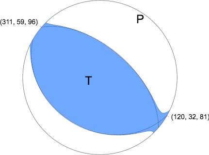
W-phase Moment Tensor (Mww)
Moment	3.711e+17 N-m
Magnitude	5.6 Mww
Depth	90.5 km
Percent DC	95 %
Half Duration	4 s
Catalog	US
Data Source	US1
Contributor	US1
Nodal Planes
Plane	Strike	Dip	Rake
NP1	311	59	96
NP2	120	32	81
Principal Axes
Axis	Value	Plunge	Azimuth
T	3.668e+17 N-m	76	238
N	0.085e+17 N-m	5	128
P	-3.753e+17 N-m	13	37
|
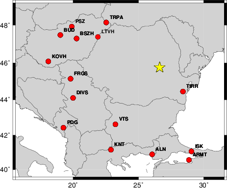
Waveform Inversion
The focal mechanism was determined using broadband seismic waveforms. The location of the event and the
and stations used for the waveform inversion are shown in the next figure.
|
|
Location of broadband stations used for waveform inversion
|
The program wvfgrd96 was used with good traces observed at short distance to determine the focal mechanism, depth and seismic moment. This technique requires a high quality signal and well determined velocity model for the Green functions. To the extent that these are the quality data, this type of mechanism should be preferred over the radiation pattern technique which requires the separate step of defining the pressure and tension quadrants and the correct strike.
The observed and predicted traces are filtered using the following gsac commands:
cut a -30 a 210
rtr
taper w 0.1
hp c 0.015 n 3
lp c 0.04 n 3
The results of this grid search from 0.5 to 19 km depth are as follow:
           DEPTH  STK   DIP  RAKE   MW    FIT
WVFGRD96    2.0    90    40   -90   4.81 0.1514
WVFGRD96    4.0    85    40   -85   4.89 0.1685
WVFGRD96    6.0    90    40   -75   4.91 0.1533
WVFGRD96    8.0   200    50   -80   4.96 0.1638
WVFGRD96   10.0   205    55   -75   4.95 0.1471
WVFGRD96   12.0   245    80   -30   4.90 0.1440
WVFGRD96   14.0    70    90    25   4.91 0.1462
WVFGRD96   16.0   245    90   -30   4.91 0.1496
WVFGRD96   18.0    65    80    25   4.92 0.1544
WVFGRD96   20.0    70    60    10   4.96 0.1620
WVFGRD96   22.0    70    55    10   4.99 0.1703
WVFGRD96   24.0    65    60    20   4.99 0.1800
WVFGRD96   26.0    65    60    20   5.01 0.1903
WVFGRD96   28.0    65    60    20   5.03 0.2009
WVFGRD96   30.0    65    55    20   5.06 0.2118
WVFGRD96   32.0    65    55    20   5.08 0.2229
WVFGRD96   34.0    65    55    20   5.10 0.2338
WVFGRD96   36.0    65    60    15   5.13 0.2449
WVFGRD96   38.0    65    60    15   5.15 0.2556
WVFGRD96   40.0    70    50    25   5.24 0.2592
WVFGRD96   42.0    70    50    30   5.26 0.2707
WVFGRD96   44.0    70    45    40   5.28 0.2825
WVFGRD96   46.0    70    45    40   5.29 0.2962
WVFGRD96   48.0    70    45    45   5.31 0.3083
WVFGRD96   50.0    75    45    50   5.33 0.3219
WVFGRD96   52.0    75    45    50   5.34 0.3351
WVFGRD96   54.0    80    45    55   5.36 0.3476
WVFGRD96   56.0    80    45    55   5.38 0.3599
WVFGRD96   58.0    85    45    60   5.39 0.3712
WVFGRD96   60.0    85    45    60   5.41 0.3822
WVFGRD96   62.0    85    45    60   5.42 0.3923
WVFGRD96   64.0    90    45    65   5.44 0.4016
WVFGRD96   66.0    90    45    65   5.45 0.4101
WVFGRD96   68.0    90    40    65   5.47 0.4186
WVFGRD96   70.0    85    45    55   5.47 0.4309
WVFGRD96   72.0    90    45    60   5.49 0.4434
WVFGRD96   74.0    95    40    60   5.51 0.4557
WVFGRD96   76.0    95    40    60   5.52 0.4676
WVFGRD96   78.0    95    40    60   5.54 0.4780
WVFGRD96   80.0    95    40    60   5.55 0.4870
WVFGRD96   82.0    95    40    60   5.55 0.4943
WVFGRD96   84.0   100    35    65   5.57 0.5002
WVFGRD96   86.0   100    35    65   5.58 0.5066
WVFGRD96   88.0   100    35    65   5.59 0.5113
WVFGRD96   90.0   100    35    65   5.60 0.5142
WVFGRD96   92.0   100    35    65   5.60 0.5155
WVFGRD96   94.0   100    35    65   5.61 0.5150
WVFGRD96   96.0   105    30    65   5.63 0.5139
WVFGRD96   98.0   105    30    65   5.63 0.5127
WVFGRD96  100.0   105    30    70   5.63 0.5099
WVFGRD96  102.0   105    30    70   5.63 0.5063
WVFGRD96  104.0   110    25    70   5.65 0.5020
WVFGRD96  106.0   110    25    70   5.65 0.4981
WVFGRD96  108.0   115    25    75   5.66 0.4934
WVFGRD96  110.0   115    25    75   5.66 0.4879
WVFGRD96  112.0   115    25    75   5.67 0.4811
WVFGRD96  114.0   115    25    75   5.67 0.4734
WVFGRD96  116.0   115    25    75   5.67 0.4649
WVFGRD96  118.0   120    20    80   5.68 0.4569
WVFGRD96  120.0   120    20    80   5.68 0.4488
WVFGRD96  122.0   120    20    80   5.68 0.4399
WVFGRD96  124.0   120    20    80   5.68 0.4303
WVFGRD96  126.0    95    25    30   5.63 0.4245
WVFGRD96  128.0    95    25    30   5.63 0.4187
The best solution is
WVFGRD96 92.0 100 35 65 5.60 0.5155
The mechanism correspond to the best fit is
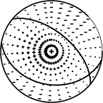
|
|
Figure 1. Waveform inversion focal mechanism
|
The best fit as a function of depth is given in the following figure:
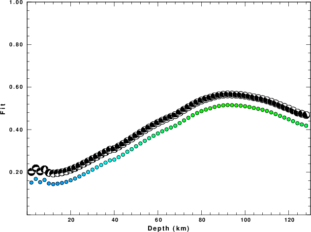
|
|
Figure 2. Depth sensitivity for waveform mechanism
|
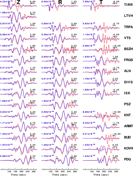
The comparison of the observed and predicted waveforms is given in the next figure. The red traces are the observed and the blue are the predicted.
Each observed-predicted component is plotted to the same scale and peak amplitudes are indicated by the numbers to the left of each trace. A pair of numbers is given in black at the right of each predicted traces. The upper number it the time shift required for maximum correlation between the observed and predicted traces. This time shift is required because the synthetics are not computed at exactly the same distance as the observed and because the velocity model used in the predictions may not be perfect.
A positive time shift indicates that the prediction is too fast and should be delayed to match the observed trace (shift to the right in this figure). A negative value indicates that the prediction is too slow. The lower number gives the percentage of variance reduction to characterize the individual goodness of fit (100% indicates a perfect fit).
The bandpass filter used in the processing and for the display was
cut a -30 a 210
rtr
taper w 0.1
hp c 0.015 n 3
lp c 0.04 n 3
|
|
Figure 3. Waveform comparison for selected depth
|
|
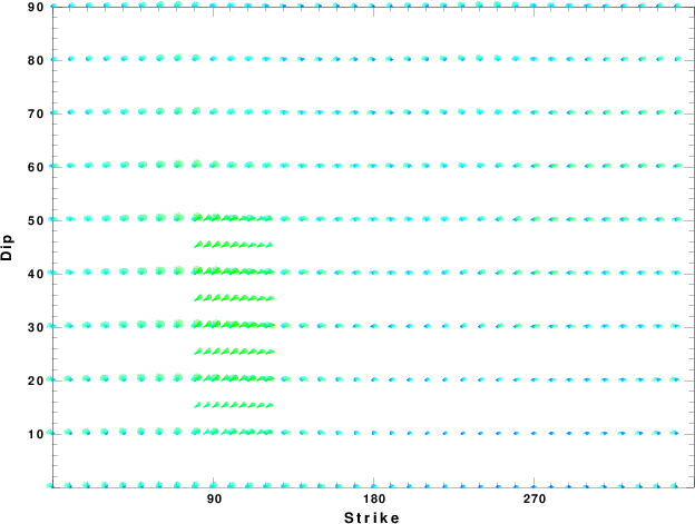
|
Focal mechanism sensitivity at the preferred depth. The red color indicates a very good fit to thewavefroms.
Each solution is plotted as a vector at a given value of strike and dip with the angle of the vector representing the rake angle, measured, with respect to the upward vertical (N) in the figure.
|
A check on the assumed source location is possible by looking at the time shifts between the observed and predicted traces. The time shifts for waveform matching arise for several reasons:
- The origin time and epicentral distance are incorrect
- The velocity model used for the inversion is incorrect
- The velocity model used to define the P-arrival time is not the
same as the velocity model used for the waveform inversion
(assuming that the initial trace alignment is based on the
P arrival time)
Assuming only a mislocation, the time shifts are fit to a functional form:
Time_shift = A + B cos Azimuth + C Sin Azimuth
The time shifts for this inversion lead to the next figure:
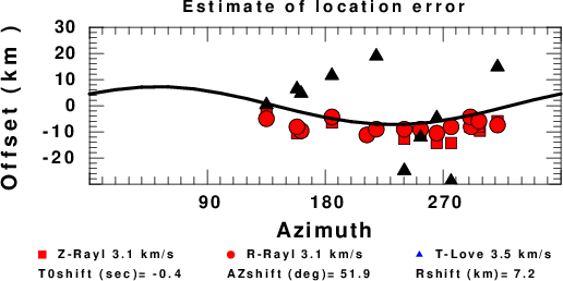
The derived shift in origin time and epicentral coordinates are given at the bottom of the figure.
Discussion
The Future
Should the national backbone of the
USGS Advanced National Seismic System (ANSS)
be implemented with an interstation separation of 300 km, it is very likely that
an earthquake such as this would have been recorded at distances on the order of
100-200 km. This means that the closest station would have information on
source depth and mechanism that was lacking here.
Acknowledgements
Dr. Harley Benz, USGS, provided the USGS USNSN digital data.
The digital data used in this study were provided by Natural Resources Canada through their AUTODRM site http://www.seismo.nrcan.gc.ca/nwfa/autodrm/autodrm_req_e.php, and IRIS using their BUD interface.
Thanks also to the many seismic network operators whose dedication make this effort possible: University of Alaska, University of Washington, Oregon State University, University of Utah, Montana Bureas of Mines, UC Berkely, Caltech, UC San Diego, Saint L ouis University, Universityof Memphis, Lamont Doehrty Earth Observatory, Boston College, the Iris stations and the Transportable Array of EarthScope.
Velocity Model
The WUS used for the waveform synthetic seismograms and for the surface wave eigenfunctions and dispersion is as follows:
MODEL.01
Model after     8 iterations
ISOTROPIC
KGS
FLAT EARTH
1-D
CONSTANT VELOCITY
LINE08
LINE09
LINE10
LINE11
      H(KM)   VP(KM/S)   VS(KM/S) RHO(GM/CC)         QP         QS       ETAP       ETAS      FREFP      FREFS
     1.9000     3.4065     2.0089     2.2150  0.302E-02  0.679E-02   0.00       0.00       1.00       1.00
     6.1000     5.5445     3.2953     2.6089  0.349E-02  0.784E-02   0.00       0.00       1.00       1.00
    13.0000     6.2708     3.7396     2.7812  0.212E-02  0.476E-02   0.00       0.00       1.00       1.00
    19.0000     6.4075     3.7680     2.8223  0.111E-02  0.249E-02   0.00       0.00       1.00       1.00
     0.0000     7.9000     4.6200     3.2760  0.164E-10  0.370E-10   0.00       0.00       1.00       1.00
Quality Control
Here we tabulate the reasons for not using certain digital data sets
The following stations did not have a valid response files:
DATE=Sat Sep 24 21:15:56 CDT 2016
Last Changed 2016/09/23