Location
2015/05/22 01:52:16 51.37 1.31 10.0 3.7 United Kingdom
Arrival Times (from USGS)
Arrival time list
Felt Map
USGS Felt map for this earthquake
USGS Felt reports archive
Focal Mechanism
 USGS/SLU Moment Tensor Solution
 ENS  2015/05/22 01:52:16:0  51.37    1.31  10.0 3.7 United Kingdom

 Stations used:
   CH.BALST CH.BOURR CH.BRANT CH.DAGMA CH.MTI02 CH.ROTHE
   EI.IWEX GB.CCA1 GB.CWF GB.DRUM GB.DYA GB.EDI GB.EDMD GB.ESK
   GB.FOEL GB.HMNX GB.HPK GB.IOMK GB.JSA GB.KESW GB.LBWR
   GB.MCH1 GB.STNC GB.WACR GB.WLF1 G.CLF G.ECH GE.IBBN GE.ILTH
   GE.WLF GR.AHRW GR.BUG

 Filtering commands used:
   cut o DIST/3.3 -30 o DIST/3.3 +70
   rtr
   taper w 0.1
   hp c 0.02 n 3
   lp c 0.06 n 3
   br c 0.12 0.25 n 4 p 2

 Best Fitting Double Couple
  Mo = 3.89e+21 dyne-cm
  Mw = 3.66
  Z  = 14 km
  Plane   Strike  Dip  Rake
   NP1      214    71    85
   NP2       50    20   105
  Principal Axes:
   Axis    Value   Plunge  Azimuth
    T   3.89e+21     64     115
    N   0.00e+00      5     216
    P  -3.89e+21     26     308

 Moment Tensor: (dyne-cm)
    Component   Value
       Mxx    -1.08e+21
       Mxy     1.25e+21
       Mxz    -1.60e+21
       Myy    -1.34e+21
       Myz     2.58e+21
       Mzz     2.42e+21


                     --------------
                 ----------------------
              -----------------------#####
             ---------------------#########
           ---   ---------------#############
          ---- P -------------###############-
         -----   -----------##################-
        -------------------###################--
        -----------------#####################--
       -----------------#######################--
       ----------------#######################---
       ---------------##########   ###########---
       --------------########### T ###########---
        ------------############   ##########---
        -----------#########################----
         ---------#########################----
          --------########################----
           ------#######################-----
             ----#####################-----
              #####################-------
                 ----########----------
                     --------------


 Global CMT Convention Moment Tensor:
      R          T          P
  2.42e+21  -1.60e+21  -2.58e+21
 -1.60e+21  -1.08e+21  -1.25e+21
 -2.58e+21  -1.25e+21  -1.34e+21


Details of the solution is found at

http://www.eas.slu.edu/eqc/eqc_mt/MECH.EU/20150522015216/index.html
|
Preferred Solution
The preferred solution from an analysis of the surface-wave spectral amplitude radiation pattern, waveform inversion and first motion observations is
      STK = 50
      DIP = 20
     RAKE = 105
       MW = 3.66
       HS = 14.0
The NDK file is 20150522015216.ndk
The waveform inversion is preferred.
Moment Tensor Comparison
The following compares this source inversion to others
| SLU |
USGSMT |
 USGS/SLU Moment Tensor Solution
 ENS  2015/05/22 01:52:16:0  51.37    1.31  10.0 3.7 United Kingdom

 Stations used:
   CH.BALST CH.BOURR CH.BRANT CH.DAGMA CH.MTI02 CH.ROTHE
   EI.IWEX GB.CCA1 GB.CWF GB.DRUM GB.DYA GB.EDI GB.EDMD GB.ESK
   GB.FOEL GB.HMNX GB.HPK GB.IOMK GB.JSA GB.KESW GB.LBWR
   GB.MCH1 GB.STNC GB.WACR GB.WLF1 G.CLF G.ECH GE.IBBN GE.ILTH
   GE.WLF GR.AHRW GR.BUG

 Filtering commands used:
   cut o DIST/3.3 -30 o DIST/3.3 +70
   rtr
   taper w 0.1
   hp c 0.02 n 3
   lp c 0.06 n 3
   br c 0.12 0.25 n 4 p 2

 Best Fitting Double Couple
  Mo = 3.89e+21 dyne-cm
  Mw = 3.66
  Z  = 14 km
  Plane   Strike  Dip  Rake
   NP1      214    71    85
   NP2       50    20   105
  Principal Axes:
   Axis    Value   Plunge  Azimuth
    T   3.89e+21     64     115
    N   0.00e+00      5     216
    P  -3.89e+21     26     308

 Moment Tensor: (dyne-cm)
    Component   Value
       Mxx    -1.08e+21
       Mxy     1.25e+21
       Mxz    -1.60e+21
       Myy    -1.34e+21
       Myz     2.58e+21
       Mzz     2.42e+21


                     --------------
                 ----------------------
              -----------------------#####
             ---------------------#########
           ---   ---------------#############
          ---- P -------------###############-
         -----   -----------##################-
        -------------------###################--
        -----------------#####################--
       -----------------#######################--
       ----------------#######################---
       ---------------##########   ###########---
       --------------########### T ###########---
        ------------############   ##########---
        -----------#########################----
         ---------#########################----
          --------########################----
           ------#######################-----
             ----#####################-----
              #####################-------
                 ----########----------
                     --------------


 Global CMT Convention Moment Tensor:
      R          T          P
  2.42e+21  -1.60e+21  -2.58e+21
 -1.60e+21  -1.08e+21  -1.25e+21
 -2.58e+21  -1.25e+21  -1.34e+21


Details of the solution is found at

http://www.eas.slu.edu/eqc/eqc_mt/MECH.EU/20150522015216/index.html
|
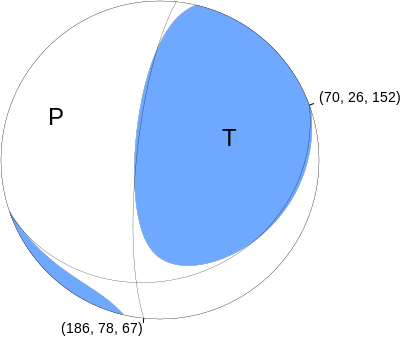
Regional Moment Tensor (Mwr)
Moment	4.298e+14 N-m
Magnitude	3.69
Depth	17.0 km
Percent DC	78%
Half Duration	–
Catalog	US (us10002bap)
Data Source	US1
Contributor	US1
Nodal Planes
Plane	Strike	Dip	Rake
NP1	186	78	67
NP2	70	26	152
Principal Axes
Axis	Value	Plunge	Azimuth
T	4.523	52	69
N	-0.495	23	191
P	-4.029	29	294
|
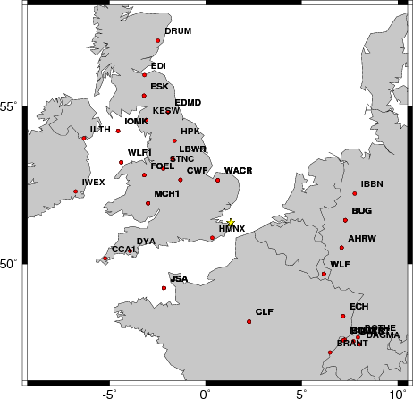
Waveform Inversion
The focal mechanism was determined using broadband seismic waveforms. The location of the event and the
and stations used for the waveform inversion are shown in the next figure.
|
|
Location of broadband stations used for waveform inversion
|
The program wvfgrd96 was used with good traces observed at short distance to determine the focal mechanism, depth and seismic moment. This technique requires a high quality signal and well determined velocity model for the Green functions. To the extent that these are the quality data, this type of mechanism should be preferred over the radiation pattern technique which requires the separate step of defining the pressure and tension quadrants and the correct strike.
The observed and predicted traces are filtered using the following gsac commands:
cut o DIST/3.3 -30 o DIST/3.3 +70
rtr
taper w 0.1
hp c 0.02 n 3
lp c 0.06 n 3
br c 0.12 0.25 n 4 p 2
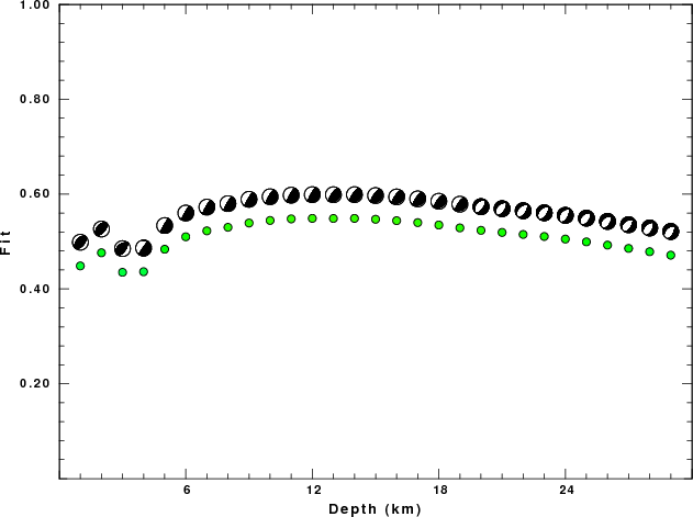
The results of this grid search from 0.5 to 19 km depth are as follow:
           DEPTH  STK   DIP  RAKE   MW    FIT
WVFGRD96    1.0    40    45    90   3.44 0.4485
WVFGRD96    2.0    40    50    90   3.51 0.4763
WVFGRD96    3.0    35    55    80   3.57 0.4350
WVFGRD96    4.0   340    10    35   3.75 0.4363
WVFGRD96    5.0   355    10    55   3.70 0.4837
WVFGRD96    6.0   210    80    85   3.67 0.5100
WVFGRD96    7.0   210    80    85   3.64 0.5225
WVFGRD96    8.0    50    10   110   3.70 0.5299
WVFGRD96    9.0   210    80    85   3.68 0.5390
WVFGRD96   10.0   210    75    85   3.68 0.5444
WVFGRD96   11.0   210    75    85   3.66 0.5477
WVFGRD96   12.0   210    75    85   3.66 0.5488
WVFGRD96   13.0   215    70    85   3.66 0.5486
WVFGRD96   14.0    50    20   105   3.66 0.5488
WVFGRD96   15.0   215    70    85   3.66 0.5469
WVFGRD96   16.0   215    70    80   3.66 0.5440
WVFGRD96   17.0   215    70    80   3.66 0.5399
WVFGRD96   18.0   215    70    80   3.66 0.5348
WVFGRD96   19.0   215    70    80   3.66 0.5287
WVFGRD96   20.0   225    30   -80   3.68 0.5235
WVFGRD96   21.0   230    35   -75   3.70 0.5192
WVFGRD96   22.0   230    35   -75   3.70 0.5149
WVFGRD96   23.0   230    35   -75   3.70 0.5106
WVFGRD96   24.0   225    35   -75   3.70 0.5052
WVFGRD96   25.0   235    40   -70   3.71 0.4992
WVFGRD96   26.0   240    40   -65   3.71 0.4924
WVFGRD96   27.0   240    40   -65   3.72 0.4854
WVFGRD96   28.0   235    40   -65   3.72 0.4785
WVFGRD96   29.0   235    40   -65   3.73 0.4712
The best solution is
WVFGRD96 14.0 50 20 105 3.66 0.5488
The mechanism correspond to the best fit is
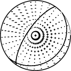
|
|
Figure 1. Waveform inversion focal mechanism
|
The best fit as a function of depth is given in the following figure:
|
|
Figure 2. Depth sensitivity for waveform mechanism
|
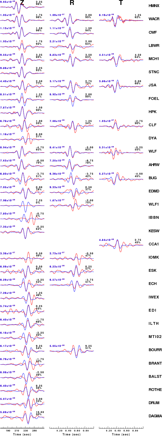
The comparison of the observed and predicted waveforms is given in the next figure. The red traces are the observed and the blue are the predicted.
Each observed-predicted component is plotted to the same scale and peak amplitudes are indicated by the numbers to the left of each trace. A pair of numbers is given in black at the right of each predicted traces. The upper number it the time shift required for maximum correlation between the observed and predicted traces. This time shift is required because the synthetics are not computed at exactly the same distance as the observed and because the velocity model used in the predictions may not be perfect.
A positive time shift indicates that the prediction is too fast and should be delayed to match the observed trace (shift to the right in this figure). A negative value indicates that the prediction is too slow. The lower number gives the percentage of variance reduction to characterize the individual goodness of fit (100% indicates a perfect fit).
The bandpass filter used in the processing and for the display was
cut o DIST/3.3 -30 o DIST/3.3 +70
rtr
taper w 0.1
hp c 0.02 n 3
lp c 0.06 n 3
br c 0.12 0.25 n 4 p 2
|
|
Figure 3. Waveform comparison for selected depth
|
|
|
Focal mechanism sensitivity at the preferred depth. The red color indicates a very good fit to thewavefroms.
Each solution is plotted as a vector at a given value of strike and dip with the angle of the vector representing the rake angle, measured, with respect to the upward vertical (N) in the figure.
|
A check on the assumed source location is possible by looking at the time shifts between the observed and predicted traces. The time shifts for waveform matching arise for several reasons:
- The origin time and epicentral distance are incorrect
- The velocity model used for the inversion is incorrect
- The velocity model used to define the P-arrival time is not the
same as the velocity model used for the waveform inversion
(assuming that the initial trace alignment is based on the
P arrival time)
Assuming only a mislocation, the time shifts are fit to a functional form:
Time_shift = A + B cos Azimuth + C Sin Azimuth
The time shifts for this inversion lead to the next figure:
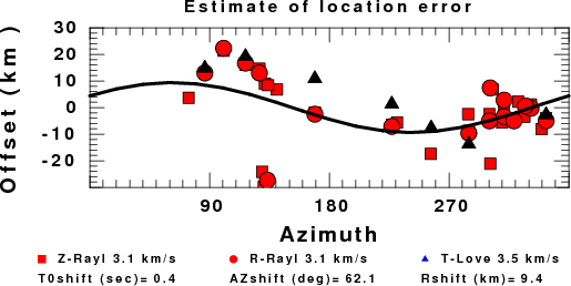
The derived shift in origin time and epicentral coordinates are given at the bottom of the figure.
Discussion
The Future
Should the national backbone of the
USGS Advanced National Seismic System (ANSS)
be implemented with an interstation separation of 300 km, it is very likely that
an earthquake such as this would have been recorded at distances on the order of
100-200 km. This means that the closest station would have information on
source depth and mechanism that was lacking here.
Acknowledgements
Dr. Harley Benz, USGS, provided the USGS USNSN digital data.
The digital data used in this study were provided by Natural Resources Canada through their AUTODRM site http://www.seismo.nrcan.gc.ca/nwfa/autodrm/autodrm_req_e.php, and IRIS using their BUD interface.
Thanks also to the many seismic network operators whose dedication make this effort possible: University of Alaska, University of Washington, Oregon State University, University of Utah, Montana Bureas of Mines, UC Berkely, Caltech, UC San Diego, Saint L ouis University, Universityof Memphis, Lamont Doehrty Earth Observatory, Boston College, the Iris stations and the Transportable Array of EarthScope.
Velocity Model
The WUS used for the waveform synthetic seismograms and for the surface wave eigenfunctions and dispersion is as follows:
MODEL.01
Model after     8 iterations
ISOTROPIC
KGS
FLAT EARTH
1-D
CONSTANT VELOCITY
LINE08
LINE09
LINE10
LINE11
      H(KM)   VP(KM/S)   VS(KM/S) RHO(GM/CC)         QP         QS       ETAP       ETAS      FREFP      FREFS
     1.9000     3.4065     2.0089     2.2150  0.302E-02  0.679E-02   0.00       0.00       1.00       1.00
     6.1000     5.5445     3.2953     2.6089  0.349E-02  0.784E-02   0.00       0.00       1.00       1.00
    13.0000     6.2708     3.7396     2.7812  0.212E-02  0.476E-02   0.00       0.00       1.00       1.00
    19.0000     6.4075     3.7680     2.8223  0.111E-02  0.249E-02   0.00       0.00       1.00       1.00
     0.0000     7.9000     4.6200     3.2760  0.164E-10  0.370E-10   0.00       0.00       1.00       1.00
Quality Control
Here we tabulate the reasons for not using certain digital data sets
The following stations did not have a valid response files:
DATE=Fri May 22 09:05:27 CDT 2015
Last Changed 2015/05/22