Location
2014/06/22 01:32:14 44.50 6.69 12 4.1 France
Arrival Times (from USGS)
Arrival time list
Felt Map
USGS Felt map for this earthquake
USGS Felt reports archive
Focal Mechanism
 USGS/SLU Moment Tensor Solution
 ENS  2014/06/22 01:32:14:0  44.50    6.69  12.0 4.1 France

 Stations used:
   CH.BNALP CH.BRANT CH.DIX CH.FIESA CH.GIMEL CH.GRIMS
   CH.HASLI CH.LAUCH CH.LLS CH.MMK CH.SENIN CH.TORNY CH.VANNI
   CH.WIMIS FR.ARBF FR.ARTF FR.BLAF FR.BSTF FR.CALF FR.GRN
   FR.ISO FR.MLYF FR.MON FR.OG02 FR.OG35 FR.OGAG FR.OGDI
   FR.OGGM FR.OGMO FR.OGS1 FR.OGS2 FR.OGS3 FR.OGSM FR.RSL
   FR.RUSF FR.SAOF FR.TRBF FR.TURF G.SSB GU.BHB GU.ENR GU.GBOS
   GU.PZZ GU.RRL GU.RSP GU.STV GU.TRAV IV.DOI IV.MONC IV.MRGE
   IV.QLNO MN.BNI RD.ORIF

 Filtering commands used:
   cut o DIST/3.3 -40 o DIST/3.3 +70
   rtr
   taper w 0.1
   hp c 0.02 n 3
   lp c 0.06 n 3

 Best Fitting Double Couple
  Mo = 1.48e+21 dyne-cm
  Mw = 3.38
  Z  = 12 km
  Plane   Strike  Dip  Rake
   NP1      143    75   -138
   NP2       40    50   -20
  Principal Axes:
   Axis    Value   Plunge  Azimuth
    T   1.48e+21     16     266
    N   0.00e+00     46     160
    P  -1.48e+21     40      10

 Moment Tensor: (dyne-cm)
    Component   Value
       Mxx    -8.43e+20
       Mxy    -6.04e+19
       Mxz    -7.41e+20
       Myy     1.34e+21
       Myz    -5.07e+20
       Mzz    -4.98e+20


                     --------------
                 ----------------------
              ##-------------------------#
             ###-------------   ----------#
           ######------------ P ----------###
          #######------------   ----------####
         #########------------------------#####
        ###########-----------------------######
        ############----------------------######
       ##############--------------------########
       ##   ###########-----------------#########
       ## T ############---------------##########
       ##   #############-------------###########
        ###################----------###########
        ####################--------############
         #####################----#############
          ####################################
           ###################----###########
             #############----------#######
              #######------------------###
                 ----------------------
                     --------------


 Global CMT Convention Moment Tensor:
      R          T          P
 -4.98e+20  -7.41e+20   5.07e+20
 -7.41e+20  -8.43e+20   6.04e+19
  5.07e+20   6.04e+19   1.34e+21


Details of the solution is found at

http://www.eas.slu.edu/eqc/eqc_mt/MECH.EU/20140622013214/index.html
|
Preferred Solution
The preferred solution from an analysis of the surface-wave spectral amplitude radiation pattern, waveform inversion and first motion observations is
      STK = 40
      DIP = 50
     RAKE = -20
       MW = 3.38
       HS = 12.0
The NDK file is 20140622013214.ndk
The waveform inversion is preferred.
Moment Tensor Comparison
The following compares this source inversion to others
| SLU |
INGVTDMT |
 USGS/SLU Moment Tensor Solution
 ENS  2014/06/22 01:32:14:0  44.50    6.69  12.0 4.1 France

 Stations used:
   CH.BNALP CH.BRANT CH.DIX CH.FIESA CH.GIMEL CH.GRIMS
   CH.HASLI CH.LAUCH CH.LLS CH.MMK CH.SENIN CH.TORNY CH.VANNI
   CH.WIMIS FR.ARBF FR.ARTF FR.BLAF FR.BSTF FR.CALF FR.GRN
   FR.ISO FR.MLYF FR.MON FR.OG02 FR.OG35 FR.OGAG FR.OGDI
   FR.OGGM FR.OGMO FR.OGS1 FR.OGS2 FR.OGS3 FR.OGSM FR.RSL
   FR.RUSF FR.SAOF FR.TRBF FR.TURF G.SSB GU.BHB GU.ENR GU.GBOS
   GU.PZZ GU.RRL GU.RSP GU.STV GU.TRAV IV.DOI IV.MONC IV.MRGE
   IV.QLNO MN.BNI RD.ORIF

 Filtering commands used:
   cut o DIST/3.3 -40 o DIST/3.3 +70
   rtr
   taper w 0.1
   hp c 0.02 n 3
   lp c 0.06 n 3

 Best Fitting Double Couple
  Mo = 1.48e+21 dyne-cm
  Mw = 3.38
  Z  = 12 km
  Plane   Strike  Dip  Rake
   NP1      143    75   -138
   NP2       40    50   -20
  Principal Axes:
   Axis    Value   Plunge  Azimuth
    T   1.48e+21     16     266
    N   0.00e+00     46     160
    P  -1.48e+21     40      10

 Moment Tensor: (dyne-cm)
    Component   Value
       Mxx    -8.43e+20
       Mxy    -6.04e+19
       Mxz    -7.41e+20
       Myy     1.34e+21
       Myz    -5.07e+20
       Mzz    -4.98e+20


                     --------------
                 ----------------------
              ##-------------------------#
             ###-------------   ----------#
           ######------------ P ----------###
          #######------------   ----------####
         #########------------------------#####
        ###########-----------------------######
        ############----------------------######
       ##############--------------------########
       ##   ###########-----------------#########
       ## T ############---------------##########
       ##   #############-------------###########
        ###################----------###########
        ####################--------############
         #####################----#############
          ####################################
           ###################----###########
             #############----------#######
              #######------------------###
                 ----------------------
                     --------------


 Global CMT Convention Moment Tensor:
      R          T          P
 -4.98e+20  -7.41e+20   5.07e+20
 -7.41e+20  -8.43e+20   6.04e+19
  5.07e+20   6.04e+19   1.34e+21


Details of the solution is found at

http://www.eas.slu.edu/eqc/eqc_mt/MECH.EU/20140622013214/index.html
|
|
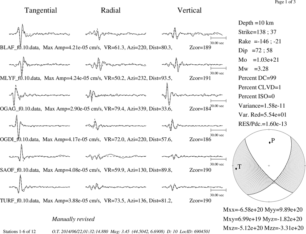
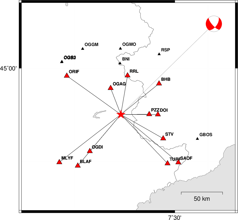
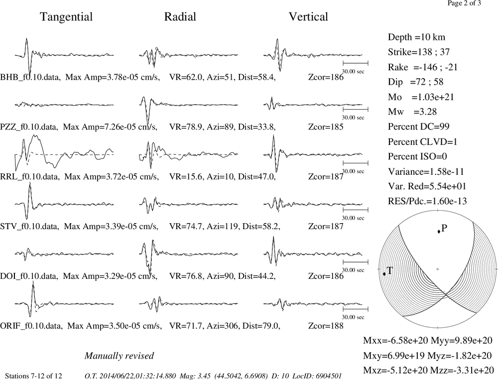
Waveform Inversion
The focal mechanism was determined using broadband seismic waveforms. The location of the event and the
and stations used for the waveform inversion are shown in the next figure.
|
|
Location of broadband stations used for waveform inversion
|
The program wvfgrd96 was used with good traces observed at short distance to determine the focal mechanism, depth and seismic moment. This technique requires a high quality signal and well determined velocity model for the Green functions. To the extent that these are the quality data, this type of mechanism should be preferred over the radiation pattern technique which requires the separate step of defining the pressure and tension quadrants and the correct strike.
The observed and predicted traces are filtered using the following gsac commands:
cut o DIST/3.3 -40 o DIST/3.3 +70
rtr
taper w 0.1
hp c 0.02 n 3
lp c 0.06 n 3
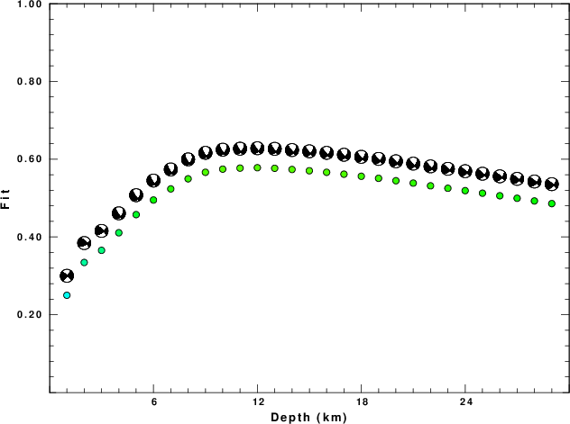
The results of this grid search from 0.5 to 19 km depth are as follow:
           DEPTH  STK   DIP  RAKE   MW    FIT
WVFGRD96    1.0    40    85     5   2.96 0.2501
WVFGRD96    2.0    65    60    35   3.14 0.3344
WVFGRD96    3.0    55    65    25   3.16 0.3656
WVFGRD96    4.0    40    40   -20   3.25 0.4108
WVFGRD96    5.0    35    40   -25   3.28 0.4574
WVFGRD96    6.0    40    45   -25   3.29 0.4950
WVFGRD96    7.0    35    45   -30   3.31 0.5236
WVFGRD96    8.0    30    40   -35   3.37 0.5495
WVFGRD96    9.0    35    45   -30   3.37 0.5663
WVFGRD96   10.0    35    45   -30   3.38 0.5744
WVFGRD96   11.0    40    50   -25   3.38 0.5770
WVFGRD96   12.0    40    50   -20   3.38 0.5781
WVFGRD96   13.0    40    50   -20   3.39 0.5766
WVFGRD96   14.0    40    50   -15   3.39 0.5735
WVFGRD96   15.0    40    55   -15   3.39 0.5703
WVFGRD96   16.0    40    55   -15   3.40 0.5663
WVFGRD96   17.0    40    55   -15   3.41 0.5614
WVFGRD96   18.0    40    55   -10   3.41 0.5561
WVFGRD96   19.0    40    55   -10   3.42 0.5508
WVFGRD96   20.0    40    55   -10   3.42 0.5446
WVFGRD96   21.0    40    55   -10   3.43 0.5385
WVFGRD96   22.0    40    55   -10   3.44 0.5315
WVFGRD96   23.0    45    55     5   3.44 0.5252
WVFGRD96   24.0    45    55     5   3.44 0.5191
WVFGRD96   25.0    45    55     5   3.45 0.5126
WVFGRD96   26.0    45    55    10   3.45 0.5060
WVFGRD96   27.0    45    55    10   3.46 0.4995
WVFGRD96   28.0    45    55    10   3.46 0.4926
WVFGRD96   29.0    45    60    10   3.46 0.4858
The best solution is
WVFGRD96 12.0 40 50 -20 3.38 0.5781
The mechanism correspond to the best fit is

|
|
Figure 1. Waveform inversion focal mechanism
|
The best fit as a function of depth is given in the following figure:
|
|
Figure 2. Depth sensitivity for waveform mechanism
|
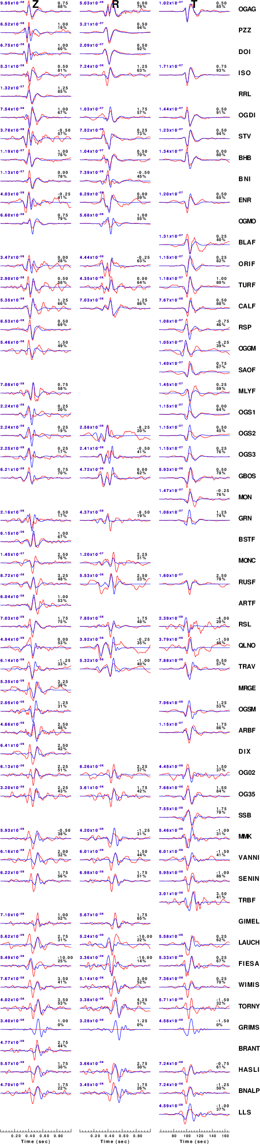
The comparison of the observed and predicted waveforms is given in the next figure. The red traces are the observed and the blue are the predicted.
Each observed-predicted component is plotted to the same scale and peak amplitudes are indicated by the numbers to the left of each trace. A pair of numbers is given in black at the right of each predicted traces. The upper number it the time shift required for maximum correlation between the observed and predicted traces. This time shift is required because the synthetics are not computed at exactly the same distance as the observed and because the velocity model used in the predictions may not be perfect.
A positive time shift indicates that the prediction is too fast and should be delayed to match the observed trace (shift to the right in this figure). A negative value indicates that the prediction is too slow. The lower number gives the percentage of variance reduction to characterize the individual goodness of fit (100% indicates a perfect fit).
The bandpass filter used in the processing and for the display was
cut o DIST/3.3 -40 o DIST/3.3 +70
rtr
taper w 0.1
hp c 0.02 n 3
lp c 0.06 n 3
|
|
Figure 3. Waveform comparison for selected depth
|
|
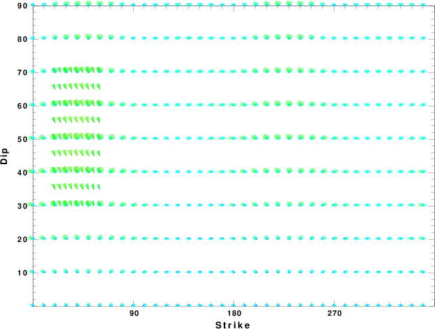
|
Focal mechanism sensitivity at the preferred depth. The red color indicates a very good fit to thewavefroms.
Each solution is plotted as a vector at a given value of strike and dip with the angle of the vector representing the rake angle, measured, with respect to the upward vertical (N) in the figure.
|
Discussion
The Future
Should the national backbone of the
USGS Advanced National Seismic System (ANSS)
be implemented with an interstation separation of 300 km, it is very likely that
an earthquake such as this would have been recorded at distances on the order of
100-200 km. This means that the closest station would have information on
source depth and mechanism that was lacking here.
Acknowledgements
Dr. Harley Benz, USGS, provided the USGS USNSN digital data.
The digital data used in this study were provided by Natural Resources Canada through their AUTODRM site http://www.seismo.nrcan.gc.ca/nwfa/autodrm/autodrm_req_e.php, and IRIS using their BUD interface.
Thanks also to the many seismic network operators whose dedication make this effort possible: University of Alaska, University of Washington, Oregon State University, University of Utah, Montana Bureas of Mines, UC Berkely, Caltech, UC San Diego, Saint L ouis University, Universityof Memphis, Lamont Doehrty Earth Observatory, Boston College, the Iris stations and the Transportable Array of EarthScope.
Velocity Model
The WUS used for the waveform synthetic seismograms and for the surface wave eigenfunctions and dispersion is as follows:
MODEL.01
Model after     8 iterations
ISOTROPIC
KGS
FLAT EARTH
1-D
CONSTANT VELOCITY
LINE08
LINE09
LINE10
LINE11
      H(KM)   VP(KM/S)   VS(KM/S) RHO(GM/CC)         QP         QS       ETAP       ETAS      FREFP      FREFS
     1.9000     3.4065     2.0089     2.2150  0.302E-02  0.679E-02   0.00       0.00       1.00       1.00
     6.1000     5.5445     3.2953     2.6089  0.349E-02  0.784E-02   0.00       0.00       1.00       1.00
    13.0000     6.2708     3.7396     2.7812  0.212E-02  0.476E-02   0.00       0.00       1.00       1.00
    19.0000     6.4075     3.7680     2.8223  0.111E-02  0.249E-02   0.00       0.00       1.00       1.00
     0.0000     7.9000     4.6200     3.2760  0.164E-10  0.370E-10   0.00       0.00       1.00       1.00
Quality Control
Here we tabulate the reasons for not using certain digital data sets
The following stations did not have a valid response files:
DATE=Wed Jun 25 05:21:13 CDT 2014
Last Changed 2014/06/22