Location

2014/06/12 11:46:48 44.683 6.783 9.5 3.40 France

Arrival Times (from USGS)

Felt Map

Focal Mechanism

SLU Moment Tensor Solution ENS 2014/06/12 11:46:48:0 44.68 6.78 9.5 3.4 France Stations used: CH.BALST CH.BERGE CH.BNALP CH.BOURR CH.BRANT CH.DIX CH.FUSIO CH.GIMEL CH.LAUCH CH.LLS CH.MMK CH.MTI02 CH.MUO CH.PANIX CH.ROTHE CH.SENIN CH.TORNY CH.VDL CH.WALHA CH.WIMIS FR.ARTF FR.CALF FR.MON FR.SAOF FR.TRBF G.ECH G.SSB GE.WLF GR.BFO GU.BHB GU.ENR GU.FINB GU.LSD GU.PCP GU.PZZ GU.REMY GU.RRL GU.RSP GU.STV IV.BOB IV.DOI IV.IMI IV.MONC IV.MRGE IV.MSSA IV.QLNO MN.BNI Filtering commands used: cut o DIST/3.3 -50 o DIST/3.3 +50 rtr taper w 0.1 hp c 0.02 n 3 lp c 0.10 n 3 Best Fitting Double Couple Mo = 1.38e+21 dyne-cm Mw = 3.36 Z = 8 km Plane Strike Dip Rake NP1 41 81 102 NP2 165 15 35 Principal Axes: Axis Value Plunge Azimuth T 1.38e+21 52 325 N 0.00e+00 12 219 P -1.38e+21 35 120 Moment Tensor: (dyne-cm) Component Value Mxx 1.20e+20 Mxy 1.54e+20 Mxz 8.78e+20 Myy -5.16e+20 Myz -9.45e+20 Mzz 3.96e+20 ############## -##################### --########################## -###########################-- --###########################----- --######### ###############------- --########## T #############---------- ---########## ############------------ --#########################------------- ---#######################---------------- ---######################----------------- ---####################------------------- ---##################--------------------- ---################----------- ------- ---##############------------- P ------- ---###########--------------- ------ ---########------------------------- ---#####-------------------------- ---#-------------------------- ####------------------------ ####------------------ ####---------- Global CMT Convention Moment Tensor: R T P 3.96e+20 8.78e+20 9.45e+20 8.78e+20 1.20e+20 -1.54e+20 9.45e+20 -1.54e+20 -5.16e+20 Details of the solution is found at http://www.eas.slu.edu/eqc/eqc_mt/MECH.IT/20140612114648/index.html

Preferred Solution

The preferred solution from an analysis of the surface-wave spectral amplitude radiation pattern, waveform inversion and first motion observations is

      STK = 165
      DIP = 15
     RAKE = 35
       MW = 3.36
       HS = 8.0

The NDK file is 20140612114648.ndk The waveform inversion is preferred.

Moment Tensor Comparison

The following compares this source inversion to others

SLU

SLU Moment Tensor Solution ENS 2014/06/12 11:46:48:0 44.68 6.78 9.5 3.4 France Stations used: CH.BALST CH.BERGE CH.BNALP CH.BOURR CH.BRANT CH.DIX CH.FUSIO CH.GIMEL CH.LAUCH CH.LLS CH.MMK CH.MTI02 CH.MUO CH.PANIX CH.ROTHE CH.SENIN CH.TORNY CH.VDL CH.WALHA CH.WIMIS FR.ARTF FR.CALF FR.MON FR.SAOF FR.TRBF G.ECH G.SSB GE.WLF GR.BFO GU.BHB GU.ENR GU.FINB GU.LSD GU.PCP GU.PZZ GU.REMY GU.RRL GU.RSP GU.STV IV.BOB IV.DOI IV.IMI IV.MONC IV.MRGE IV.MSSA IV.QLNO MN.BNI Filtering commands used: cut o DIST/3.3 -50 o DIST/3.3 +50 rtr taper w 0.1 hp c 0.02 n 3 lp c 0.10 n 3 Best Fitting Double Couple Mo = 1.38e+21 dyne-cm Mw = 3.36 Z = 8 km Plane Strike Dip Rake NP1 41 81 102 NP2 165 15 35 Principal Axes: Axis Value Plunge Azimuth T 1.38e+21 52 325 N 0.00e+00 12 219 P -1.38e+21 35 120 Moment Tensor: (dyne-cm) Component Value Mxx 1.20e+20 Mxy 1.54e+20 Mxz 8.78e+20 Myy -5.16e+20 Myz -9.45e+20 Mzz 3.96e+20 ############## -##################### --########################## -###########################-- --###########################----- --######### ###############------- --########## T #############---------- ---########## ############------------ --#########################------------- ---#######################---------------- ---######################----------------- ---####################------------------- ---##################--------------------- ---################----------- ------- ---##############------------- P ------- ---###########--------------- ------ ---########------------------------- ---#####-------------------------- ---#-------------------------- ####------------------------ ####------------------ ####---------- Global CMT Convention Moment Tensor: R T P 3.96e+20 8.78e+20 9.45e+20 8.78e+20 1.20e+20 -1.54e+20 9.45e+20 -1.54e+20 -5.16e+20 Details of the solution is found at http://www.eas.slu.edu/eqc/eqc_mt/MECH.IT/20140612114648/index.html

Waveform Inversion

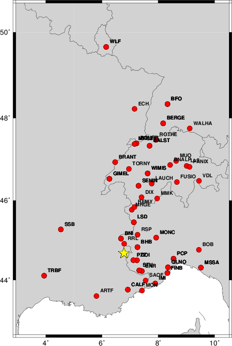
The focal mechanism was determined using broadband seismic waveforms. The location of the event and the and stations used for the waveform inversion are shown in the next figure.

Location of broadband stations used for waveform inversion

The program wvfgrd96 was used with good traces observed at short distance to determine the focal mechanism, depth and seismic moment. This technique requires a high quality signal and well determined velocity model for the Green functions. To the extent that these are the quality data, this type of mechanism should be preferred over the radiation pattern technique which requires the separate step of defining the pressure and tension quadrants and the correct strike.

The observed and predicted traces are filtered using the following gsac commands:

cut o DIST/3.3 -50 o DIST/3.3 +50
rtr
taper w 0.1
hp c 0.02 n 3 
lp c 0.10 n 3

The results of this grid search from 0.5 to 19 km depth are as follow:

           DEPTH  STK   DIP  RAKE   MW    FIT
WVFGRD96    1.0   225    35   -90   3.21 0.4474
WVFGRD96    2.0   220    25   -95   3.29 0.4065
WVFGRD96    3.0   105     5   -25   3.30 0.4890
WVFGRD96    4.0   130    10     0   3.27 0.5664
WVFGRD96    5.0   135     5     5   3.39 0.6260
WVFGRD96    6.0   150    10    20   3.39 0.6778
WVFGRD96    7.0   155    10    25   3.40 0.7064
WVFGRD96    8.0   165    15    35   3.36 0.7183
WVFGRD96    9.0   165    15    35   3.37 0.7180
WVFGRD96   10.0   160    20    30   3.38 0.7099
WVFGRD96   11.0   155    20    25   3.39 0.6960
WVFGRD96   12.0   155    20    25   3.40 0.6786
WVFGRD96   13.0   155    20    25   3.40 0.6588
WVFGRD96   14.0   155    20    25   3.41 0.6388
WVFGRD96   15.0   155    20    20   3.45 0.6190
WVFGRD96   16.0   150    20    15   3.46 0.5966
WVFGRD96   17.0   150    20    15   3.47 0.5736
WVFGRD96   18.0   145    20    10   3.48 0.5505
WVFGRD96   19.0   145    20    10   3.48 0.5270
WVFGRD96   20.0   145    20    10   3.49 0.5038
WVFGRD96   21.0   145    20    10   3.50 0.4799
WVFGRD96   22.0   145    20    10   3.50 0.4561
WVFGRD96   23.0   145    20    10   3.51 0.4332
WVFGRD96   24.0   140    20     5   3.51 0.4118
WVFGRD96   25.0   140    20     5   3.51 0.3934
WVFGRD96   26.0   140    20     5   3.52 0.3780
WVFGRD96   27.0   150    20    15   3.52 0.3673
WVFGRD96   28.0   160    20    25   3.52 0.3600
WVFGRD96   29.0   165    25    35   3.53 0.3565

The best solution is

WVFGRD96    8.0   165    15    35   3.36 0.7183

The mechanism correspond to the best fit is

Figure 1. Waveform inversion focal mechanism

The best fit as a function of depth is given in the following figure:

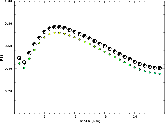
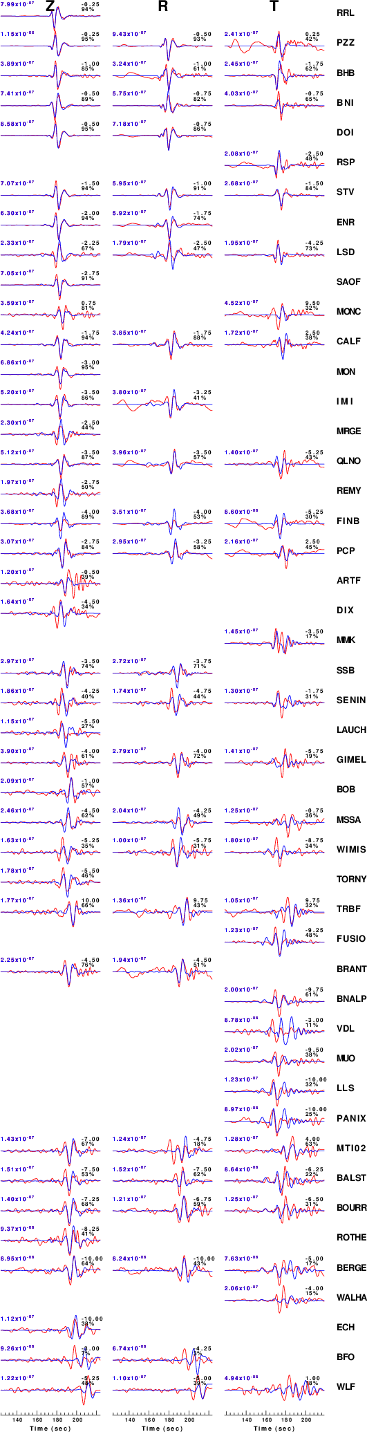
Figure 2. Depth sensitivity for waveform mechanism

The comparison of the observed and predicted waveforms is given in the next figure. The red traces are the observed and the blue are the predicted. Each observed-predicted component is plotted to the same scale and peak amplitudes are indicated by the numbers to the left of each trace. A pair of numbers is given in black at the right of each predicted traces. The upper number it the time shift required for maximum correlation between the observed and predicted traces. This time shift is required because the synthetics are not computed at exactly the same distance as the observed and because the velocity model used in the predictions may not be perfect. A positive time shift indicates that the prediction is too fast and should be delayed to match the observed trace (shift to the right in this figure). A negative value indicates that the prediction is too slow. The lower number gives the percentage of variance reduction to characterize the individual goodness of fit (100% indicates a perfect fit).

The bandpass filter used in the processing and for the display was

cut o DIST/3.3 -50 o DIST/3.3 +50
rtr
taper w 0.1
hp c 0.02 n 3 
lp c 0.10 n 3

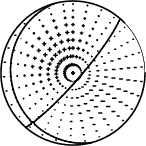
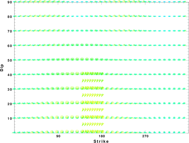
Figure 3. Waveform comparison for selected depth. Red: observed; Blue - predicted. The time shift with respect to the model prediction is indicated. The percent of fit is also indicated.

Focal mechanism sensitivity at the preferred depth. The red color indicates a very good fit to thewavefroms. Each solution is plotted as a vector at a given value of strike and dip with the angle of the vector representing the rake angle, measured, with respect to the upward vertical (N) in the figure.

A check on the assumed source location is possible by looking at the time shifts between the observed and predicted traces. The time shifts for waveform matching arise for several reasons:

The origin time and epicentral distance are incorrect
The velocity model used for the inversion is incorrect
The velocity model used to define the P-arrival time is not the same as the velocity model used for the waveform inversion (assuming that the initial trace alignment is based on the P arrival time)

Assuming only a mislocation, the time shifts are fit to a functional form:

 Time_shift = A + B cos Azimuth + C Sin Azimuth

The time shifts for this inversion lead to the next figure:

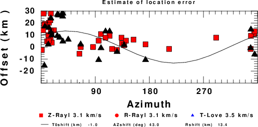
The derived shift in origin time and epicentral coordinates are given at the bottom of the figure.

Discussion

Velocity Model

The nnCIA used for the waveform synthetic seismograms and for the surface wave eigenfunctions and dispersion is as follows:

MODEL.01
C.It. A. Di Luzio et al Earth Plan Lettrs 280 (2009) 1-12 Fig 5. 7-8 MODEL/SURF3
ISOTROPIC
KGS
FLAT EARTH
1-D
CONSTANT VELOCITY
LINE08
LINE09
LINE10
LINE11
      H(KM)   VP(KM/S)   VS(KM/S) RHO(GM/CC)         QP         QS       ETAP       ETAS      FREFP      FREFS
     1.5000     3.7497     2.1436     2.2753  0.500E-02  0.100E-01   0.00       0.00       1.00       1.00    
     3.0000     4.9399     2.8210     2.4858  0.500E-02  0.100E-01   0.00       0.00       1.00       1.00    
     3.0000     6.0129     3.4336     2.7058  0.500E-02  0.100E-01   0.00       0.00       1.00       1.00    
     7.0000     5.5516     3.1475     2.6093  0.167E-02  0.333E-02   0.00       0.00       1.00       1.00    
    15.0000     5.8805     3.3583     2.6770  0.167E-02  0.333E-02   0.00       0.00       1.00       1.00    
     6.0000     7.1059     4.0081     3.0002  0.167E-02  0.333E-02   0.00       0.00       1.00       1.00    
     8.0000     7.1000     3.9864     3.0120  0.167E-02  0.333E-02   0.00       0.00       1.00       1.00    
     0.0000     7.9000     4.4036     3.2760  0.167E-02  0.333E-02   0.00       0.00       1.00       1.00

Quality Control

Here we tabulate the reasons for not using certain digital data sets

The following stations did not have a valid response files:

DATE=Thu Jun 12 08:40:42 CDT 2014

Last Changed 2014/06/12