Location
SLU Location
The program elocate was used with the WUS model listed below to locate this event. The reason for this effort is that the EMSC location was fixed at a depth of 2.0 km, and because of the difference in source depths from the various moment tensor solutions.
The output of the elocate run is in elocate.txt. The takeoff angles are used with the SLU moment tensor solution to plot the first motions in the comparison given below. The similarity in depth between the SLU location and the SLU moment tensor provides some confidence in the SLU MT depth.
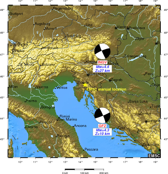
EMSC Location
2014/04/22 08:58:27 45.65 14.26 2.0 4.5 Slovenia
Arrival Times (from USGS)
Arrival time list
Felt Map
USGS Felt map for this earthquake
USGS Felt reports archive
Focal Mechanism
 USGS/SLU Moment Tensor Solution
 ENS  2014/04/22 08:58:27:0  45.65   14.26   2.0 4.5 Slovenia

 Stations used:
   CH.BERNI CH.BNALP CH.DAVOX CH.FUORN CH.FUSIO CH.LIENZ
   CH.LLS CH.MUO CH.PANIX CH.PLONS CH.SLE CH.VDL CH.WILA
   CH.ZUR GR.FUR GR.GEC2 GR.UBR HU.BEHE HU.MORH HU.PSZ HU.SOP
   IV.BRMO IV.FVI IV.STAL MN.BLY MN.PDG MN.TIR MN.TRI MN.TUE
   OE.ABTA OE.ARSA OE.CONA OE.CSNA OE.DAVA OE.FETA OE.KBA
   OE.MOA OE.OBKA OE.RETA OE.SOKA SJ.BBLS SJ.FRGS SL.BOJS
   SL.CADS SL.CRES SL.CRNS SL.GBAS SL.GORS SL.JAVS SL.KNDS
   SL.KOGS SL.LJU SL.MOZS SL.PERS SL.ROBS SL.VISS SL.VNDS
   SL.VOJS

 Filtering commands used:
   cut a -20 a 180
   rtr
   taper w 0.1
   hp c 0.02 n 3
   lp c 0.06 n 3

 Best Fitting Double Couple
  Mo = 4.84e+22 dyne-cm
  Mw = 4.39
  Z  = 17 km
  Plane   Strike  Dip  Rake
   NP1      335    90   -175
   NP2      245    85     0
  Principal Axes:
   Axis    Value   Plunge  Azimuth
    T   4.84e+22      4     110
    N   0.00e+00     85     335
    P  -4.84e+22      4     200

 Moment Tensor: (dyne-cm)
    Component   Value
       Mxx    -3.69e+22
       Mxy    -3.10e+22
       Mxz     1.78e+21
       Myy     3.69e+22
       Myz     3.82e+21
       Mzz     0.00e+00


                     --------------
                 ###-------------------
              #######---------------------
             #########---------------------
           ###########-----------------------
          #############-----------------------
         ###############---------------------##
        #################---------------########
        ##################---------#############
       ####################----##################
       ####################-#####################
       ################-----#####################
       ############----------####################
        ########--------------###############
        #####------------------############## T
         #----------------------#############
          -----------------------#############
           -----------------------###########
             ---------------------#########
              ---------------------#######
                 ---   -------------###
                     P ------------


 Global CMT Convention Moment Tensor:
      R          T          P
  0.00e+00   1.78e+21  -3.82e+21
  1.78e+21  -3.69e+22   3.10e+22
 -3.82e+21   3.10e+22   3.69e+22


Details of the solution is found at

http://www.eas.slu.edu/eqc/eqc_mt/MECH.EU/20140422085827/index.html
|
Preferred Solution
The preferred solution from an analysis of the surface-wave spectral amplitude radiation pattern, waveform inversion and first motion observations is
      STK = 245
      DIP = 85
     RAKE = 0
       MW = 4.39
       HS = 17.0
The NDK file is 20140422085827.ndk
The waveform inversion is preferred.
Moment Tensor Comparison
The following compares this source inversion to others
| SLU |
SLUFM |
EMSC |
INGVTDMT |
QRCMT |
 USGS/SLU Moment Tensor Solution
 ENS  2014/04/22 08:58:27:0  45.65   14.26   2.0 4.5 Slovenia

 Stations used:
   CH.BERNI CH.BNALP CH.DAVOX CH.FUORN CH.FUSIO CH.LIENZ
   CH.LLS CH.MUO CH.PANIX CH.PLONS CH.SLE CH.VDL CH.WILA
   CH.ZUR GR.FUR GR.GEC2 GR.UBR HU.BEHE HU.MORH HU.PSZ HU.SOP
   IV.BRMO IV.FVI IV.STAL MN.BLY MN.PDG MN.TIR MN.TRI MN.TUE
   OE.ABTA OE.ARSA OE.CONA OE.CSNA OE.DAVA OE.FETA OE.KBA
   OE.MOA OE.OBKA OE.RETA OE.SOKA SJ.BBLS SJ.FRGS SL.BOJS
   SL.CADS SL.CRES SL.CRNS SL.GBAS SL.GORS SL.JAVS SL.KNDS
   SL.KOGS SL.LJU SL.MOZS SL.PERS SL.ROBS SL.VISS SL.VNDS
   SL.VOJS

 Filtering commands used:
   cut a -20 a 180
   rtr
   taper w 0.1
   hp c 0.02 n 3
   lp c 0.06 n 3

 Best Fitting Double Couple
  Mo = 4.84e+22 dyne-cm
  Mw = 4.39
  Z  = 17 km
  Plane   Strike  Dip  Rake
   NP1      335    90   -175
   NP2      245    85     0
  Principal Axes:
   Axis    Value   Plunge  Azimuth
    T   4.84e+22      4     110
    N   0.00e+00     85     335
    P  -4.84e+22      4     200

 Moment Tensor: (dyne-cm)
    Component   Value
       Mxx    -3.69e+22
       Mxy    -3.10e+22
       Mxz     1.78e+21
       Myy     3.69e+22
       Myz     3.82e+21
       Mzz     0.00e+00


                     --------------
                 ###-------------------
              #######---------------------
             #########---------------------
           ###########-----------------------
          #############-----------------------
         ###############---------------------##
        #################---------------########
        ##################---------#############
       ####################----##################
       ####################-#####################
       ################-----#####################
       ############----------####################
        ########--------------###############
        #####------------------############## T
         #----------------------#############
          -----------------------#############
           -----------------------###########
             ---------------------#########
              ---------------------#######
                 ---   -------------###
                     P ------------


 Global CMT Convention Moment Tensor:
      R          T          P
  0.00e+00   1.78e+21  -3.82e+21
  1.78e+21  -3.69e+22   3.10e+22
 -3.82e+21   3.10e+22   3.69e+22


Details of the solution is found at

http://www.eas.slu.edu/eqc/eqc_mt/MECH.EU/20140422085827/index.html
|
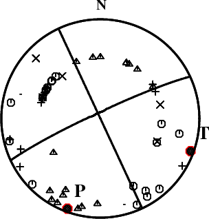
First motions and takeoff angles from an elocate run.
|
EMSC Quick MT Solutions
|
|
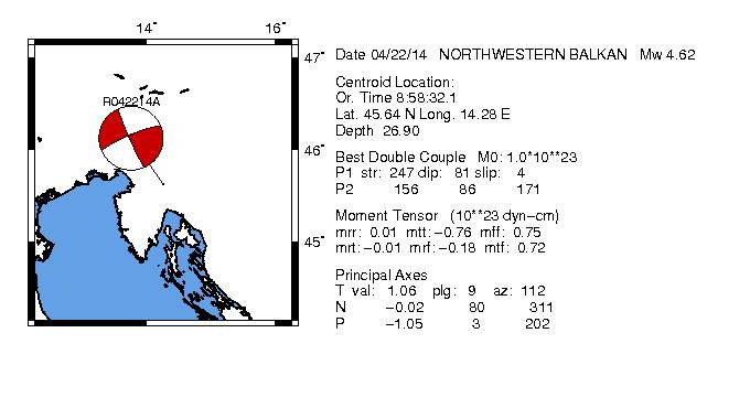
CENTROID, MOMENT TENSOR SOLUTION
HARVARD EVENT-FILE NAME S042214A
DATA USED: GSN
SURFACE WAVES:   24S, 37C, T= 35
CENTROID LOCATION:
ORIGIN TIME       08:58:32.1 0.3
LAT 45.64N 0.02;LON  14.28E 0.02
DEP  26.9 1.2;HALF-DURATION  1.1
MOMENT TENSOR; SCALE 10**23 D-CM
  MRR= 0.01 0.08; MTT=-0.76 0.06
  MPP= 0.75 0.05; MRT=-0.01 0.07
  MRP=-0.18 0.06; MTP= 0.72 0.04
 PRINCIPAL AXES:
 1.(T) VAL=  1.06;PLG= 9;AZM=112
 2.(N)      -0.02;    80;    311
 3.(P)      -1.05;     3;    202
BEST DOUBLE COUPLE:M0=1.1*10**23
 NP1:STRIKE=247;DIP=81;SLIP=   4
 NP2:STRIKE=156;DIP=86;SLIP= 171

            -----------
        ###----------------
      ######-----------------
    #########------------------
   ##########-------------------
  ############-------------------
  #############----------########
 ##############-----##############
 ##############-##################
 ##########------#################
 #######----------################
  ###--------------###########
  -----------------########### T
   -----------------##########
    -----------------##########
      ----------------#######
        --   ----------####
           P ----------


 http://autorcmt.bo.ingv.it/QRCMT-on-line/E1404220858A.html
|
Waveform Inversion
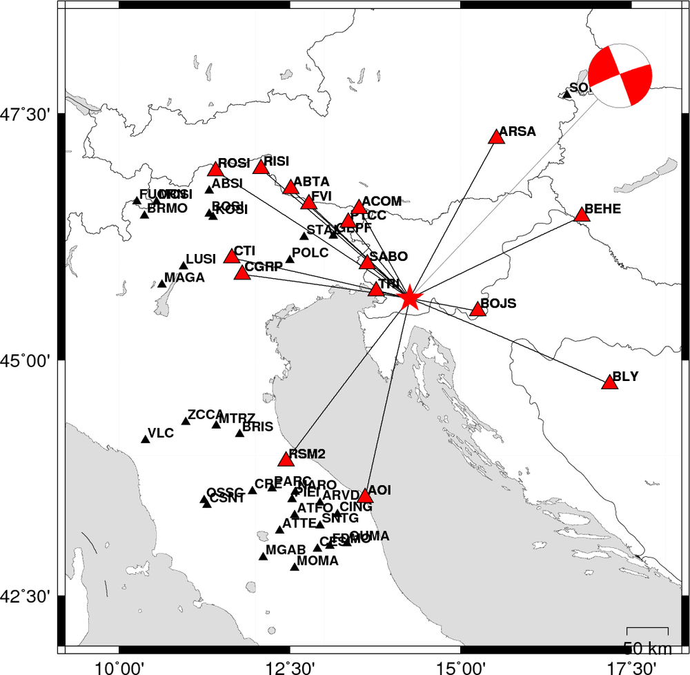
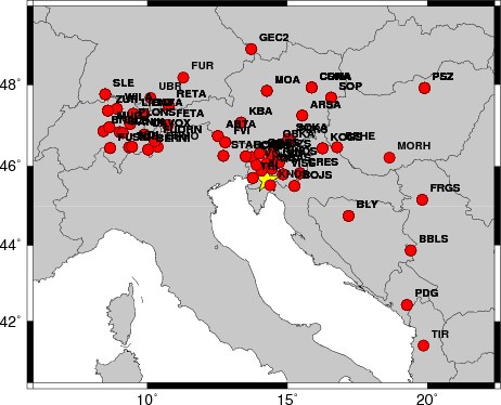
The focal mechanism was determined using broadband seismic waveforms. The location of the event and the
and stations used for the waveform inversion are shown in the next figure.
|
|
Location of broadband stations used for waveform inversion
|
The program wvfgrd96 was used with good traces observed at short distance to determine the focal mechanism, depth and seismic moment. This technique requires a high quality signal and well determined velocity model for the Green functions. To the extent that these are the quality data, this type of mechanism should be preferred over the radiation pattern technique which requires the separate step of defining the pressure and tension quadrants and the correct strike.
The observed and predicted traces are filtered using the following gsac commands:
cut a -20 a 180
rtr
taper w 0.1
hp c 0.02 n 3
lp c 0.06 n 3
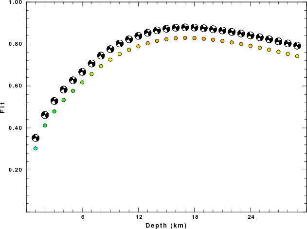
The results of this grid search from 0.5 to 19 km depth are as follow:
           DEPTH  STK   DIP  RAKE   MW    FIT
WVFGRD96    1.0   245    80   -10   3.92 0.3025
WVFGRD96    2.0   245    75   -10   4.05 0.4119
WVFGRD96    3.0   245    70   -10   4.11 0.4785
WVFGRD96    4.0   245    70   -10   4.16 0.5330
WVFGRD96    5.0   245    70   -10   4.19 0.5770
WVFGRD96    6.0   245    75   -10   4.21 0.6171
WVFGRD96    7.0   245    75   -10   4.24 0.6568
WVFGRD96    8.0   245    75   -10   4.28 0.6946
WVFGRD96    9.0   245    75    -5   4.29 0.7254
WVFGRD96   10.0   245    75    -5   4.31 0.7521
WVFGRD96   11.0   245    80    -5   4.33 0.7722
WVFGRD96   12.0   245    80    -5   4.34 0.7887
WVFGRD96   13.0   245    80    -5   4.35 0.8032
WVFGRD96   14.0   245    80    -5   4.36 0.8147
WVFGRD96   15.0   245    80     0   4.37 0.8224
WVFGRD96   16.0   245    85     0   4.38 0.8274
WVFGRD96   17.0   245    85     0   4.39 0.8290
WVFGRD96   18.0   245    85     0   4.40 0.8279
WVFGRD96   19.0   245    85     0   4.41 0.8249
WVFGRD96   20.0   245    85     0   4.41 0.8202
WVFGRD96   21.0   245    85     0   4.42 0.8143
WVFGRD96   22.0   245    85     0   4.43 0.8073
WVFGRD96   23.0   245    85     0   4.43 0.7996
WVFGRD96   24.0   245    85     0   4.44 0.7909
WVFGRD96   25.0   245    85     0   4.44 0.7817
WVFGRD96   26.0   245    85     0   4.45 0.7725
WVFGRD96   27.0   245    85     0   4.45 0.7625
WVFGRD96   28.0   245    80     0   4.45 0.7524
WVFGRD96   29.0   245    80     0   4.46 0.7421
The best solution is
WVFGRD96 17.0 245 85 0 4.39 0.8290
The mechanism correspond to the best fit is
|
|
Figure 1. Waveform inversion focal mechanism
|
The best fit as a function of depth is given in the following figure:
|
|
Figure 2. Depth sensitivity for waveform mechanism
|
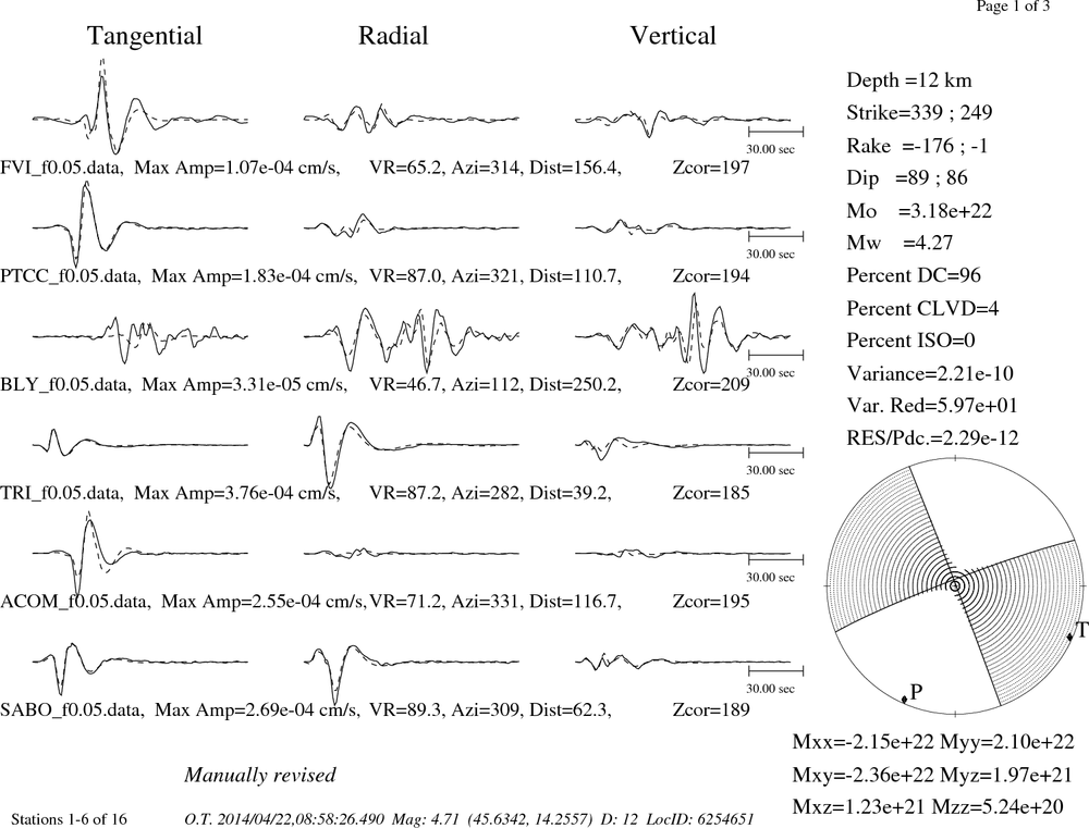
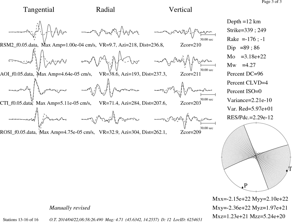
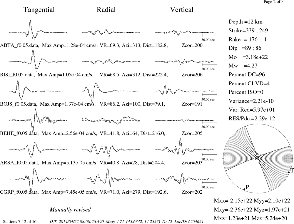
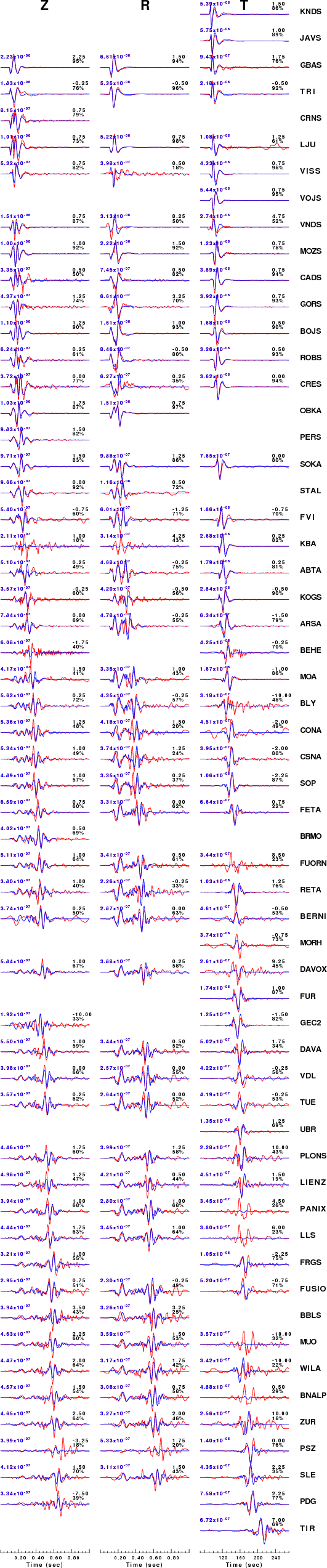
The comparison of the observed and predicted waveforms is given in the next figure. The red traces are the observed and the blue are the predicted.
Each observed-predicted component is plotted to the same scale and peak amplitudes are indicated by the numbers to the left of each trace. A pair of numbers is given in black at the right of each predicted traces. The upper number it the time shift required for maximum correlation between the observed and predicted traces. This time shift is required because the synthetics are not computed at exactly the same distance as the observed and because the velocity model used in the predictions may not be perfect.
A positive time shift indicates that the prediction is too fast and should be delayed to match the observed trace (shift to the right in this figure). A negative value indicates that the prediction is too slow. The lower number gives the percentage of variance reduction to characterize the individual goodness of fit (100% indicates a perfect fit).
The bandpass filter used in the processing and for the display was
cut a -20 a 180
rtr
taper w 0.1
hp c 0.02 n 3
lp c 0.06 n 3
|
|
Figure 3. Waveform comparison for selected depth
|
|
|
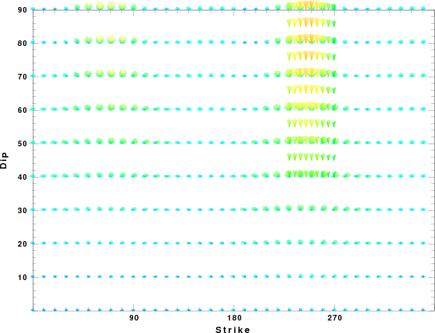
Focal mechanism sensitivity at the preferred depth. The red color indicates a very good fit to thewavefroms.
Each solution is plotted as a vector at a given value of strike and dip with the angle of the vector representing the rake angle, measured, with respect to the upward vertical (N) in the figure.
|
A check on the assumed source location is possible by looking at the time shifts between the observed and predicted traces. The time shifts for waveform matching arise for several reasons:
- The origin time and epicentral distance are incorrect
- The velocity model used for the inversion is incorrect
- The velocity model used to define the P-arrival time is not the
same as the velocity model used for the waveform inversion
(assuming that the initial trace alignment is based on the
P arrival time)
Assuming only a mislocation, the time shifts are fit to a functional form:
Time_shift = A + B cos Azimuth + C Sin Azimuth
The time shifts for this inversion lead to the next figure:
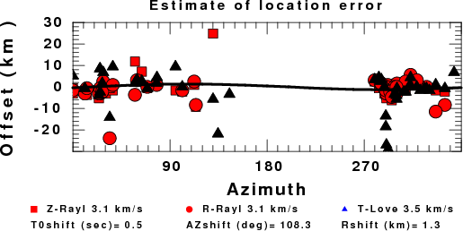
The derived shift in origin time and epicentral coordinates are given at the bottom of the figure.
Discussion
The Future
Should the national backbone of the
USGS Advanced National Seismic System (ANSS)
be implemented with an interstation separation of 300 km, it is very likely that
an earthquake such as this would have been recorded at distances on the order of
100-200 km. This means that the closest station would have information on
source depth and mechanism that was lacking here.
Acknowledgements
Dr. Harley Benz, USGS, provided the USGS USNSN digital data.
The digital data used in this study were provided by Natural Resources Canada through their AUTODRM site http://www.seismo.nrcan.gc.ca/nwfa/autodrm/autodrm_req_e.php, and IRIS using their BUD interface.
Thanks also to the many seismic network operators whose dedication make this effort possible: University of Alaska, University of Washington, Oregon State University, University of Utah, Montana Bureas of Mines, UC Berkely, Caltech, UC San Diego, Saint L ouis University, Universityof Memphis, Lamont Doehrty Earth Observatory, Boston College, the Iris stations and the Transportable Array of EarthScope.
Velocity Model
The WUS used for the waveform synthetic seismograms and for the surface wave eigenfunctions and dispersion is as follows:
MODEL.01
Model after     8 iterations
ISOTROPIC
KGS
FLAT EARTH
1-D
CONSTANT VELOCITY
LINE08
LINE09
LINE10
LINE11
      H(KM)   VP(KM/S)   VS(KM/S) RHO(GM/CC)         QP         QS       ETAP       ETAS      FREFP      FREFS
     1.9000     3.4065     2.0089     2.2150  0.302E-02  0.679E-02   0.00       0.00       1.00       1.00
     6.1000     5.5445     3.2953     2.6089  0.349E-02  0.784E-02   0.00       0.00       1.00       1.00
    13.0000     6.2708     3.7396     2.7812  0.212E-02  0.476E-02   0.00       0.00       1.00       1.00
    19.0000     6.4075     3.7680     2.8223  0.111E-02  0.249E-02   0.00       0.00       1.00       1.00
     0.0000     7.9000     4.6200     3.2760  0.164E-10  0.370E-10   0.00       0.00       1.00       1.00
Quality Control
Here we tabulate the reasons for not using certain digital data sets
The following stations did not have a valid response files:
DATE=Tue Apr 22 21:34:23 CDT 2014
Last Changed 2014/04/22