2014/03/13 17:31:59 45.77 14.79 2.0 4.4 Slovenia
USGS Felt map for this earthquake
 USGS/SLU Moment Tensor Solution
 ENS  2014/03/13 17:31:59:0  45.77   14.79   2.0 4.4 Slovenia

 Stations used:
   HU.SOP IV.FVI IV.PTCC OE.ABTA OE.ARSA OE.CONA OE.CSNA
   OE.KBA OE.MOA OE.MYKA OE.OBKA SL.BOJS SL.CADS SL.CEY
   SL.CRNS SL.DOBS SL.GBAS SL.GCIS SL.GORS SL.JAVS SL.KNDS
   SL.KOGS SL.LJU SL.MOZS SL.PERS

 Filtering commands used:
   cut a -20 a 110
   rtr
   taper w 0.1
   hp c 0.03 n 3
   lp c 0.10 n 3

 Best Fitting Double Couple
  Mo = 1.66e+22 dyne-cm
  Mw = 4.08
  Z  = 2 km
  Plane   Strike  Dip  Rake
   NP1      265    50    80
   NP2      100    41   102
  Principal Axes:
   Axis    Value   Plunge  Azimuth
    T   1.66e+22     81     122
    N   0.00e+00      8     271
    P  -1.66e+22      5       2

 Moment Tensor: (dyne-cm)
    Component   Value
       Mxx    -1.64e+22
       Mxy    -7.77e+20
       Mxz    -2.67e+21
       Myy     2.61e+20
       Myz     2.09e+21
       Mzz     1.61e+22


                     ------ P -----
                 ----------   ---------
              ----------------------------
             ------------------------------
           ----------------------------------
          ------------------------------------
         ----------#####################-------
        -------#############################----
        -----#################################--
       #---#####################################-
       #-###################   ##################
       #-################### T ##################
       ----#################   ##################
        ----####################################
        ------################################--
         -------############################---
          ----------#####################-----
           ---------------#########----------
             ------------------------------
              ----------------------------
                 ----------------------
                     --------------


 Global CMT Convention Moment Tensor:
      R          T          P
  1.61e+22  -2.67e+21  -2.09e+21
 -2.67e+21  -1.64e+22   7.77e+20
 -2.09e+21   7.77e+20   2.61e+20


Details of the solution is found at

http://www.eas.slu.edu/eqc/eqc_mt/MECH.EU/20140313173159/index.html
|
      STK = 265
      DIP = 50
     RAKE = 80
       MW = 4.08
       HS = 2.0
The NDK file is 20140313173159.ndk Traces were noisy because of earlier event in Japan. The initial search wanted a shallow depth, but the WUS Green's functions had significant hsort period surface waves not seen in the data. So I decided to use the CUS model.
The following compares this source inversion to others
 USGS/SLU Moment Tensor Solution
 ENS  2014/03/13 17:31:59:0  45.77   14.79   2.0 4.4 Slovenia

 Stations used:
   HU.SOP IV.FVI IV.PTCC OE.ABTA OE.ARSA OE.CONA OE.CSNA
   OE.KBA OE.MOA OE.MYKA OE.OBKA SL.BOJS SL.CADS SL.CEY
   SL.CRNS SL.DOBS SL.GBAS SL.GCIS SL.GORS SL.JAVS SL.KNDS
   SL.KOGS SL.LJU SL.MOZS SL.PERS

 Filtering commands used:
   cut a -20 a 110
   rtr
   taper w 0.1
   hp c 0.03 n 3
   lp c 0.10 n 3

 Best Fitting Double Couple
  Mo = 1.66e+22 dyne-cm
  Mw = 4.08
  Z  = 2 km
  Plane   Strike  Dip  Rake
   NP1      265    50    80
   NP2      100    41   102
  Principal Axes:
   Axis    Value   Plunge  Azimuth
    T   1.66e+22     81     122
    N   0.00e+00      8     271
    P  -1.66e+22      5       2

 Moment Tensor: (dyne-cm)
    Component   Value
       Mxx    -1.64e+22
       Mxy    -7.77e+20
       Mxz    -2.67e+21
       Myy     2.61e+20
       Myz     2.09e+21
       Mzz     1.61e+22


                     ------ P -----
                 ----------   ---------
              ----------------------------
             ------------------------------
           ----------------------------------
          ------------------------------------
         ----------#####################-------
        -------#############################----
        -----#################################--
       #---#####################################-
       #-###################   ##################
       #-################### T ##################
       ----#################   ##################
        ----####################################
        ------################################--
         -------############################---
          ----------#####################-----
           ---------------#########----------
             ------------------------------
              ----------------------------
                 ----------------------
                     --------------


 Global CMT Convention Moment Tensor:
      R          T          P
  1.61e+22  -2.67e+21  -2.09e+21
 -2.67e+21  -1.64e+22   7.77e+20
 -2.09e+21   7.77e+20   2.61e+20


Details of the solution is found at

http://www.eas.slu.edu/eqc/eqc_mt/MECH.EU/20140313173159/index.html
|
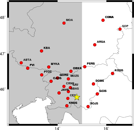
The focal mechanism was determined using broadband seismic waveforms. The location of the event and the and stations used for the waveform inversion are shown in the next figure.
|
|
|
|
The program wvfgrd96 was used with good traces observed at short distance to determine the focal mechanism, depth and seismic moment. This technique requires a high quality signal and well determined velocity model for the Green functions. To the extent that these are the quality data, this type of mechanism should be preferred over the radiation pattern technique which requires the separate step of defining the pressure and tension quadrants and the correct strike.
The observed and predicted traces are filtered using the following gsac commands:
cut a -20 a 110
rtr
taper w 0.1
hp c 0.03 n 3
lp c 0.10 n 3
The results of this grid search from 0.5 to 19 km depth are as follow:
           DEPTH  STK   DIP  RAKE   MW    FIT
WVFGRD96    0.5   245    55    55   3.95 0.3877
WVFGRD96    1.0   255    50    65   4.00 0.4101
WVFGRD96    2.0   265    50    80   4.08 0.4211
WVFGRD96    3.0   270    55    85   4.10 0.3708
WVFGRD96    4.0    40    65   -25   3.99 0.3370
WVFGRD96    5.0   225    70   -30   4.00 0.3444
WVFGRD96    6.0   225    65   -30   4.02 0.3553
WVFGRD96    7.0   225    65   -30   4.03 0.3657
WVFGRD96    8.0   225    65   -30   4.04 0.3745
WVFGRD96    9.0   225    65   -30   4.05 0.3819
WVFGRD96   10.0   220    60   -35   4.08 0.3848
WVFGRD96   11.0   220    60   -35   4.08 0.3888
WVFGRD96   12.0   220    55   -35   4.10 0.3919
WVFGRD96   13.0   220    55   -35   4.11 0.3934
WVFGRD96   14.0   220    55   -35   4.12 0.3928
WVFGRD96   15.0   220    55   -35   4.13 0.3902
WVFGRD96   16.0   220    55   -35   4.13 0.3863
WVFGRD96   17.0   220    55   -35   4.14 0.3815
WVFGRD96   18.0   220    55   -35   4.15 0.3760
WVFGRD96   19.0   220    55   -35   4.15 0.3698
WVFGRD96   20.0   290    55   -65   4.19 0.3667
WVFGRD96   21.0   295    55   -65   4.20 0.3653
WVFGRD96   22.0   290    50   -70   4.21 0.3640
WVFGRD96   23.0   290    50   -70   4.22 0.3616
WVFGRD96   24.0   295    50   -65   4.23 0.3584
WVFGRD96   25.0   295    50   -65   4.23 0.3551
WVFGRD96   26.0   295    50   -65   4.24 0.3514
WVFGRD96   27.0   295    50   -65   4.25 0.3471
WVFGRD96   28.0   295    50   -60   4.25 0.3427
WVFGRD96   29.0   295    50   -60   4.25 0.3369
The best solution is
WVFGRD96 2.0 265 50 80 4.08 0.4211
The mechanism correspond to the best fit is
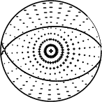
|
|
|
The best fit as a function of depth is given in the following figure:
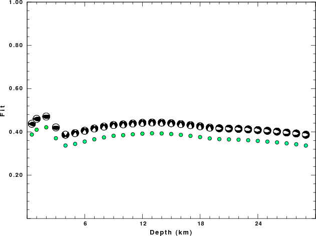
|
|
|
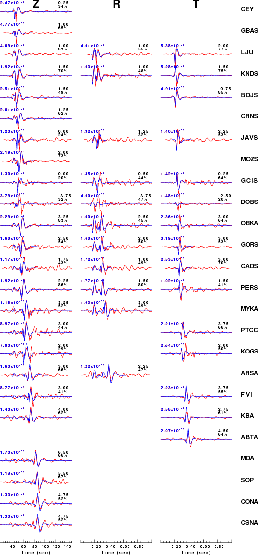
The comparison of the observed and predicted waveforms is given in the next figure. The red traces are the observed and the blue are the predicted. Each observed-predicted component is plotted to the same scale and peak amplitudes are indicated by the numbers to the left of each trace. A pair of numbers is given in black at the right of each predicted traces. The upper number it the time shift required for maximum correlation between the observed and predicted traces. This time shift is required because the synthetics are not computed at exactly the same distance as the observed and because the velocity model used in the predictions may not be perfect. A positive time shift indicates that the prediction is too fast and should be delayed to match the observed trace (shift to the right in this figure). A negative value indicates that the prediction is too slow. The lower number gives the percentage of variance reduction to characterize the individual goodness of fit (100% indicates a perfect fit).
The bandpass filter used in the processing and for the display was
cut a -20 a 110
rtr
taper w 0.1
hp c 0.03 n 3
lp c 0.10 n 3
|
|
|
|
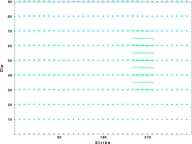
| Focal mechanism sensitivity at the preferred depth. The red color indicates a very good fit to thewavefroms. Each solution is plotted as a vector at a given value of strike and dip with the angle of the vector representing the rake angle, measured, with respect to the upward vertical (N) in the figure. |
A check on the assumed source location is possible by looking at the time shifts between the observed and predicted traces. The time shifts for waveform matching arise for several reasons:
Time_shift = A + B cos Azimuth + C Sin Azimuth
The time shifts for this inversion lead to the next figure:
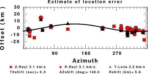
The derived shift in origin time and epicentral coordinates are given at the bottom of the figure.
Should the national backbone of the USGS Advanced National Seismic System (ANSS) be implemented with an interstation separation of 300 km, it is very likely that an earthquake such as this would have been recorded at distances on the order of 100-200 km. This means that the closest station would have information on source depth and mechanism that was lacking here.
Dr. Harley Benz, USGS, provided the USGS USNSN digital data. The digital data used in this study were provided by Natural Resources Canada through their AUTODRM site http://www.seismo.nrcan.gc.ca/nwfa/autodrm/autodrm_req_e.php, and IRIS using their BUD interface.
Thanks also to the many seismic network operators whose dedication make this effort possible: University of Alaska, University of Washington, Oregon State University, University of Utah, Montana Bureas of Mines, UC Berkely, Caltech, UC San Diego, Saint L ouis University, Universityof Memphis, Lamont Doehrty Earth Observatory, Boston College, the Iris stations and the Transportable Array of EarthScope.
The CUS used for the waveform synthetic seismograms and for the surface wave eigenfunctions and dispersion is as follows:
MODEL.01
CUS Model with Q from simple gamma values
ISOTROPIC
KGS
FLAT EARTH
1-D
CONSTANT VELOCITY
LINE08
LINE09
LINE10
LINE11
  H(KM) VP(KM/S) VS(KM/S) RHO(GM/CC)   QP   QS  ETAP  ETAS  FREFP  FREFS
  1.0000  5.0000  2.8900  2.5000 0.172E-02 0.387E-02 0.00  0.00  1.00  1.00
  9.0000  6.1000  3.5200  2.7300 0.160E-02 0.363E-02 0.00  0.00  1.00  1.00
 10.0000  6.4000  3.7000  2.8200 0.149E-02 0.336E-02 0.00  0.00  1.00  1.00
 20.0000  6.7000  3.8700  2.9020 0.000E-04 0.000E-04 0.00  0.00  1.00  1.00
  0.0000  8.1500  4.7000  3.3640 0.194E-02 0.431E-02 0.00  0.00  1.00  1.00
Here we tabulate the reasons for not using certain digital data sets
The following stations did not have a valid response files:
DATE=Fri Mar 14 08:16:33 CDT 2014