Location

2013/06/05 18:45:46 47.97 19.24 10.0 4.10 Hungary

The elocate solution is given in elocate.txt. We ran this solution to check the location and to make the first motion plot. The first motion plot was made assuming a fixed source depth of 10 km, and has the waveform inversion nodal planes superimposed.

Arrival Times (from USGS)

Arrival time list

Felt Map

USGS Felt map for this earthquake

USGS Felt reports archive

Focal Mechanism

USGS/SLU Moment Tensor Solution ENS 2013/06/05 18:45:46:0 47.97 19.24 10.0 4.1 Hungary Stations used: CZ.DPC CZ.JAVC CZ.KHC CZ.KRUC CZ.NKC CZ.OKC CZ.TREC CZ.VRAC GE.MORC GE.PSZ GE.RUE GR.BRG GR.CLL GR.GEC2 GR.GRA1 GR.WET HU.BUD HU.SOP MN.BLY MN.PDG MN.VTS NI.ACOM NI.CIMO NI.CLUD NI.DRE NI.FUSE NI.PRED NI.SABO NI.ZOU2 OE.ARSA OE.CONA OE.CSNA OE.KBA OE.MOA OE.MYKA OE.OBKA OE.SOKA PL.BEL PL.GKP PL.KSP PL.NIE PL.OJC RO.BUR31 RO.BZS SL.BOJS SL.CADS SL.CEY SL.CRES SL.CRNS SL.GBAS SL.GORS SL.JAVS SL.KNDS SL.KOGS SL.LJU SL.MOZS SL.PERS SL.ROBS SL.SKDS SL.VISS SL.VNDS SL.VOJS SX.TANN Filtering commands used: hp c 0.02 n 3 lp c 0.10 n 3 br c 0.12 0.25 n 4 p 2 Best Fitting Double Couple Mo = 7.00e+21 dyne-cm Mw = 3.83 Z = 6 km Plane Strike Dip Rake NP1 80 90 10 NP2 350 80 180 Principal Axes: Axis Value Plunge Azimuth T 7.00e+21 7 305 N 0.00e+00 80 80 P -7.00e+21 7 215 Moment Tensor: (dyne-cm) Component Value Mxx -2.36e+21 Mxy -6.48e+21 Mxz 1.20e+21 Myy 2.36e+21 Myz -2.11e+20 Mzz -1.06e+14 ####---------- #########------------- #############--------------- #############---------------- T ##############----------------- # ##############------------------ ####################------------------ #####################------------------- ######################------------------ #######################--------------##### #######################---################ ################--------################## #####-------------------################## -----------------------################# ------------------------################ -----------------------############### ----------------------############## ---------------------############# -- --------------########### - P --------------########## --------------####### -----------### Global CMT Convention Moment Tensor: R T P -1.06e+14 1.20e+21 2.11e+20 1.20e+21 -2.36e+21 6.48e+21 2.11e+20 6.48e+21 2.36e+21 Details of the solution is found at http://www.eas.slu.edu/eqc/eqc_mt/MECH.EU/20130605184546/index.html

Preferred Solution

      STK = 80
      DIP = 90
     RAKE = 10
       MW = 3.83
       HS = 6.0

Surprisingly, depth control was difficult for this strike-slip event. Perhaps this is because it was shallow and also because it was necessary to remove the shorter period information using a microseism filter. The elocate epicenter agrees well with the EMSC solution.

Moment Tensor Comparison

The following compares this source inversion to others

SLU

SLUFM

USGS/SLU Moment Tensor Solution ENS 2013/06/05 18:45:46:0 47.97 19.24 10.0 4.1 Hungary Stations used: CZ.DPC CZ.JAVC CZ.KHC CZ.KRUC CZ.NKC CZ.OKC CZ.TREC CZ.VRAC GE.MORC GE.PSZ GE.RUE GR.BRG GR.CLL GR.GEC2 GR.GRA1 GR.WET HU.BUD HU.SOP MN.BLY MN.PDG MN.VTS NI.ACOM NI.CIMO NI.CLUD NI.DRE NI.FUSE NI.PRED NI.SABO NI.ZOU2 OE.ARSA OE.CONA OE.CSNA OE.KBA OE.MOA OE.MYKA OE.OBKA OE.SOKA PL.BEL PL.GKP PL.KSP PL.NIE PL.OJC RO.BUR31 RO.BZS SL.BOJS SL.CADS SL.CEY SL.CRES SL.CRNS SL.GBAS SL.GORS SL.JAVS SL.KNDS SL.KOGS SL.LJU SL.MOZS SL.PERS SL.ROBS SL.SKDS SL.VISS SL.VNDS SL.VOJS SX.TANN Filtering commands used: hp c 0.02 n 3 lp c 0.10 n 3 br c 0.12 0.25 n 4 p 2 Best Fitting Double Couple Mo = 7.00e+21 dyne-cm Mw = 3.83 Z = 6 km Plane Strike Dip Rake NP1 80 90 10 NP2 350 80 180 Principal Axes: Axis Value Plunge Azimuth T 7.00e+21 7 305 N 0.00e+00 80 80 P -7.00e+21 7 215 Moment Tensor: (dyne-cm) Component Value Mxx -2.36e+21 Mxy -6.48e+21 Mxz 1.20e+21 Myy 2.36e+21 Myz -2.11e+20 Mzz -1.06e+14 ####---------- #########------------- #############--------------- #############---------------- T ##############----------------- # ##############------------------ ####################------------------ #####################------------------- ######################------------------ #######################--------------##### #######################---################ ################--------################## #####-------------------################## -----------------------################# ------------------------################ -----------------------############### ----------------------############## ---------------------############# -- --------------########### - P --------------########## --------------####### -----------### Global CMT Convention Moment Tensor: R T P -1.06e+14 1.20e+21 2.11e+20 1.20e+21 -2.36e+21 6.48e+21 2.11e+20 6.48e+21 2.36e+21 Details of the solution is found at http://www.eas.slu.edu/eqc/eqc_mt/MECH.EU/20130605184546/index.html

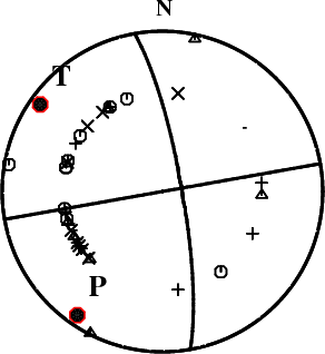
First motions and takeoff angles from an elocate run.

Waveform Inversion

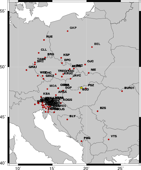
The focal mechanism was determined using broadband seismic waveforms. The location of the event and the and stations used for the waveform inversion are shown in the next figure.

Location of broadband stations used for waveform inversion

The program wvfgrd96 was used with good traces observed at short distance to determine the focal mechanism, depth and seismic moment. This technique requires a high quality signal and well determined velocity model for the Green functions. To the extent that these are the quality data, this type of mechanism should be preferred over the radiation pattern technique which requires the separate step of defining the pressure and tension quadrants and the correct strike.

The observed and predicted traces are filtered using the following gsac commands:

hp c 0.02 n 3
lp c 0.10 n 3
br c 0.12 0.25 n 4 p 2

           DEPTH  STK   DIP  RAKE   MW    FIT
WVFGRD96    0.5   255    90     0   3.43 0.2550
WVFGRD96    1.0    75    90     0   3.49 0.2959
WVFGRD96    2.0    80    90     0   3.66 0.4911
WVFGRD96    3.0    80    90     0   3.73 0.5702
WVFGRD96    4.0    80    90     5   3.78 0.6106
WVFGRD96    5.0   260    90   -10   3.81 0.6276
WVFGRD96    6.0    80    90    10   3.83 0.6312
WVFGRD96    7.0   260    90   -10   3.86 0.6286
WVFGRD96    8.0   260    85   -20   3.88 0.6289
WVFGRD96    9.0   260    75   -15   3.89 0.6192
WVFGRD96   10.0   260    75   -15   3.91 0.6151
WVFGRD96   11.0   260    75   -15   3.92 0.6110
WVFGRD96   12.0   260    70   -15   3.93 0.6076
WVFGRD96   13.0   265    65   -10   3.92 0.6042
WVFGRD96   14.0   265    70   -10   3.93 0.6044
WVFGRD96   15.0   265    70   -10   3.94 0.6045
WVFGRD96   16.0   265    70   -15   3.95 0.6047
WVFGRD96   17.0   265    70   -15   3.96 0.6049
WVFGRD96   18.0   265    70   -15   3.97 0.6051
WVFGRD96   19.0   265    70   -15   3.98 0.6044
WVFGRD96   20.0   265    70   -15   3.99 0.6030
WVFGRD96   21.0   265    70   -15   4.00 0.6020
WVFGRD96   22.0   265    70   -15   4.00 0.6007
WVFGRD96   23.0   265    65   -20   4.01 0.5987
WVFGRD96   24.0   265    70   -20   4.02 0.5961
WVFGRD96   25.0   265    65   -20   4.02 0.5949
WVFGRD96   26.0   265    70   -25   4.03 0.5929
WVFGRD96   27.0   265    70   -25   4.03 0.5902
WVFGRD96   28.0   265    70   -25   4.04 0.5874
WVFGRD96   29.0   265    70   -25   4.05 0.5858

The best solution is

WVFGRD96    6.0    80    90    10   3.83 0.6312

The mechanism correspond to the best fit is

Figure 1. Waveform inversion focal mechanism

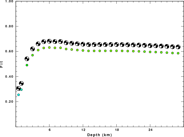
The best fit as a function of depth is given in the following figure:

Figure 2. Depth sensitivity for waveform mechanism

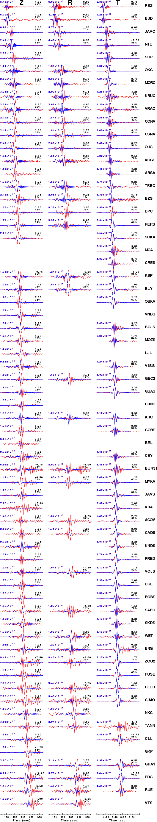
The comparison of the observed and predicted waveforms is given in the next figure. The red traces are the observed and the blue are the predicted. Each observed-predicted component is plotted to the same scale and peak amplitudes are indicated by the numbers to the left of each trace. A pair of numbers is given in black at the right of each predicted traces. The upper number it the time shift required for maximum correlation between the observed and predicted traces. This time shift is required because the synthetics are not computed at exactly the same distance as the observed and because the velocity model used in the predictions may not be perfect. A positive time shift indicates that the prediction is too fast and should be delayed to match the observed trace (shift to the right in this figure). A negative value indicates that the prediction is too slow. The lower number gives the percentage of variance reduction to characterize the individual goodness of fit (100% indicates a perfect fit).

The bandpass filter used in the processing and for the display was

hp c 0.02 n 3
lp c 0.10 n 3
br c 0.12 0.25 n 4 p 2

Figure 3. Waveform comparison for selected depth

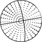
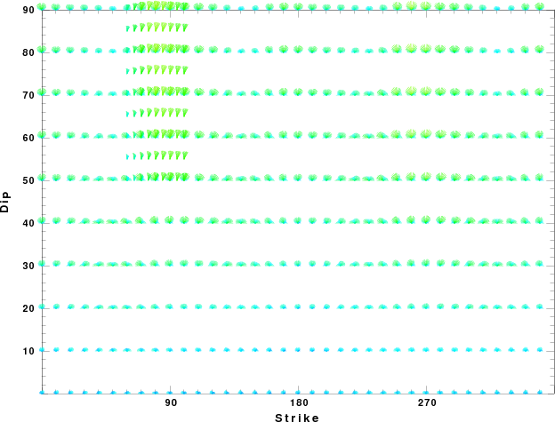
Focal mechanism sensitivity at the preferred depth. The red color indicates a very good fit to thewavefroms. Each solution is plotted as a vector at a given value of strike and dip with the angle of the vector representing the rake angle, measured, with respect to the upward vertical (N) in the figure.

A check on the assumed source location is possible by looking at the time shifts between the observed and predicted traces. The time shifts for waveform matching arise for several reasons:

• The origin time and epicentral distance are incorrect
• The velocity model used for the inversion is incorrect
• The velocity model used to define the P-arrival time is not the same as the velocity model used for the waveform inversion (assuming that the initial trace alignment is based on the P arrival time)

 Time_shift = A + B cos Azimuth + C Sin Azimuth

The time shifts for this inversion lead to the next figure:

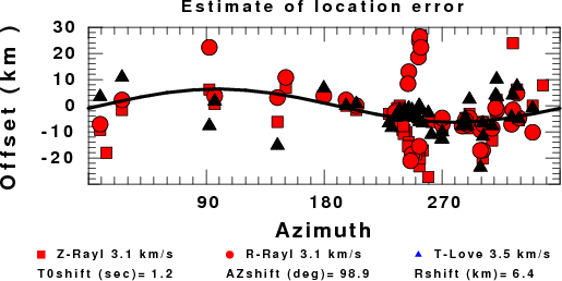
The derived shift in origin time and epicentral coordinates are given at the bottom of the figure.

Discussion

The Future

Should the national backbone of the USGS Advanced National Seismic System (ANSS) be implemented with an interstation separation of 300 km, it is very likely that an earthquake such as this would have been recorded at distances on the order of 100-200 km. This means that the closest station would have information on source depth and mechanism that was lacking here.

Acknowledgements

Dr. Harley Benz, USGS, provided the USGS USNSN digital data. The digital data used in this study were provided by Natural Resources Canada through their AUTODRM site http://www.seismo.nrcan.gc.ca/nwfa/autodrm/autodrm_req_e.php, and IRIS using their BUD interface.

Thanks also to the many seismic network operators whose dedication make this effort possible: University of Alaska, University of Washington, Oregon State University, University of Utah, Montana Bureas of Mines, UC Berkely, Caltech, UC San Diego, Saint L ouis University, Universityof Memphis, Lamont Doehrty Earth Observatory, Boston College, the Iris stations and the Transportable Array of EarthScope.

Velocity Model

The WUS used for the waveform synthetic seismograms and for the surface wave eigenfunctions and dispersion is as follows:

MODEL.01
Model after     8 iterations
ISOTROPIC
KGS
FLAT EARTH
1-D
CONSTANT VELOCITY
LINE08
LINE09
LINE10
LINE11
      H(KM)   VP(KM/S)   VS(KM/S) RHO(GM/CC)         QP         QS       ETAP       ETAS      FREFP      FREFS
     1.9000     3.4065     2.0089     2.2150  0.302E-02  0.679E-02   0.00       0.00       1.00       1.00    
     6.1000     5.5445     3.2953     2.6089  0.349E-02  0.784E-02   0.00       0.00       1.00       1.00    
    13.0000     6.2708     3.7396     2.7812  0.212E-02  0.476E-02   0.00       0.00       1.00       1.00    
    19.0000     6.4075     3.7680     2.8223  0.111E-02  0.249E-02   0.00       0.00       1.00       1.00    
     0.0000     7.9000     4.6200     3.2760  0.164E-10  0.370E-10   0.00       0.00       1.00       1.00    

Quality Control

Here we tabulate the reasons for not using certain digital data sets

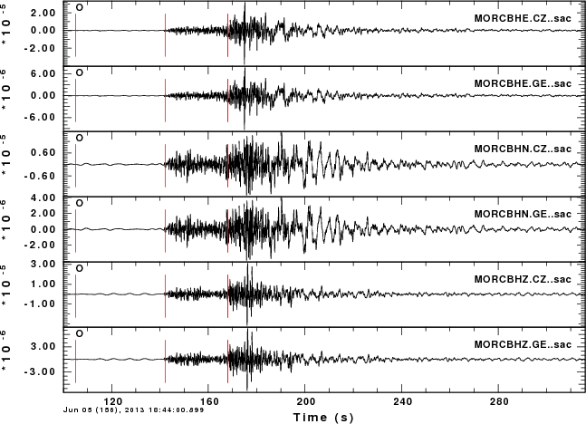
The following stations did not have a valid response files:

There are two data systems at MORC. The as seen in the next figure shows the ground velocity in units of m/s for the three channels of the GE and CZ networks. The CZ network ground motions are a factor of 4 greater than those of the GE network data set. Since the GE traces agree with all others used in the source inversion, the conclusion is that the metadata for the MORC-CZ channels is not correct.

The polezero files obtained from the GFZ data center are as follow:

• SAC_PZs_CZ_MORC_BHZ__2013.156.18.43.37.1950_2013.156.18.56.58.4195
• SAC_PZs_GE_MORC_BHZ__2013.156.18.43.37.1950_2013.156.18.56.58.4195