2013/05/28 00:09:52 43.22 41.58 2.0 5.20 Georgia
USGS Felt map for this earthquake
 USGS/SLU Moment Tensor Solution
 ENS  2013/05/28 00:09:52:0  43.22   41.58   2.0 5.2 Georgia

 Stations used:
   GE.CSS GE.ISP GO.AKH GO.BATM GO.BGD IU.GNI IU.KIEV RO.CFR
   RO.IAS

 Filtering commands used:
   hp c 0.02 n 3
   lp c 0.05 n 3

 Best Fitting Double Couple
  Mo = 5.07e+23 dyne-cm
  Mw = 5.07
  Z  = 23 km
  Plane   Strike  Dip  Rake
   NP1      130    73   121
   NP2      245    35    30
  Principal Axes:
   Axis    Value   Plunge  Azimuth
    T   5.07e+23     51      76
    N   0.00e+00     30     300
    P  -5.07e+23     22     196

 Moment Tensor: (dyne-cm)
    Component   Value
       Mxx    -3.89e+23
       Mxy    -7.06e+22
       Mxz     2.31e+23
       Myy     1.50e+23
       Myz     2.89e+23
       Mzz     2.38e+23


                     --------------
                 ----------------------
              ----------------------------
             --------------###########-----
           ##---------#####################--
          ###------##########################-
         ######-###############################
        ######--################################
        #####----###################   #########
       #####-------################# T ##########
       ####----------###############   ##########
       ###-------------##########################
       ###---------------########################
        #------------------#####################
        #--------------------###################
         -----------------------###############
          -------------------------###########
           ----------------------------######
             ---------   ------------------
              -------- P -----------------
                 -----   --------------
                     --------------


 Global CMT Convention Moment Tensor:
      R          T          P
  2.38e+23   2.31e+23  -2.89e+23
  2.31e+23  -3.89e+23   7.06e+22
 -2.89e+23   7.06e+22   1.50e+23


Details of the solution is found at

http://www.eas.slu.edu/eqc/eqc_mt/MECH.EU/20130528000952/index.html
|
      STK = 245
      DIP = 35
     RAKE = 30
       MW = 5.07
       HS = 23.0
The waveform inversion is preferred.
The following compares this source inversion to others
 USGS/SLU Moment Tensor Solution
 ENS  2013/05/28 00:09:52:0  43.22   41.58   2.0 5.2 Georgia

 Stations used:
   GE.CSS GE.ISP GO.AKH GO.BATM GO.BGD IU.GNI IU.KIEV RO.CFR
   RO.IAS

 Filtering commands used:
   hp c 0.02 n 3
   lp c 0.05 n 3

 Best Fitting Double Couple
  Mo = 5.07e+23 dyne-cm
  Mw = 5.07
  Z  = 23 km
  Plane   Strike  Dip  Rake
   NP1      130    73   121
   NP2      245    35    30
  Principal Axes:
   Axis    Value   Plunge  Azimuth
    T   5.07e+23     51      76
    N   0.00e+00     30     300
    P  -5.07e+23     22     196

 Moment Tensor: (dyne-cm)
    Component   Value
       Mxx    -3.89e+23
       Mxy    -7.06e+22
       Mxz     2.31e+23
       Myy     1.50e+23
       Myz     2.89e+23
       Mzz     2.38e+23


                     --------------
                 ----------------------
              ----------------------------
             --------------###########-----
           ##---------#####################--
          ###------##########################-
         ######-###############################
        ######--################################
        #####----###################   #########
       #####-------################# T ##########
       ####----------###############   ##########
       ###-------------##########################
       ###---------------########################
        #------------------#####################
        #--------------------###################
         -----------------------###############
          -------------------------###########
           ----------------------------######
             ---------   ------------------
              -------- P -----------------
                 -----   --------------
                     --------------


 Global CMT Convention Moment Tensor:
      R          T          P
  2.38e+23   2.31e+23  -2.89e+23
  2.31e+23  -3.89e+23   7.06e+22
 -2.89e+23   7.06e+22   1.50e+23


Details of the solution is found at

http://www.eas.slu.edu/eqc/eqc_mt/MECH.EU/20130528000952/index.html
|
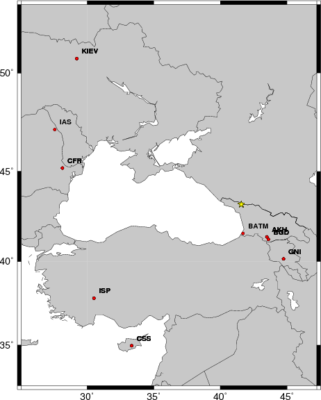
The focal mechanism was determined using broadband seismic waveforms. The location of the event and the and stations used for the waveform inversion are shown in the next figure.
|
|
|
|
The program wvfgrd96 was used with good traces observed at short distance to determine the focal mechanism, depth and seismic moment. This technique requires a high quality signal and well determined velocity model for the Green functions. To the extent that these are the quality data, this type of mechanism should be preferred over the radiation pattern technique which requires the separate step of defining the pressure and tension quadrants and the correct strike.
The observed and predicted traces are filtered using the following gsac commands:
hp c 0.02 n 3
lp c 0.05 n 3
The results of this grid search from 0.5 to 19 km depth are as follow:
           DEPTH  STK   DIP  RAKE   MW    FIT
WVFGRD96    0.5   310    55   -65   4.71 0.3270
WVFGRD96    1.0   300    50   -70   4.73 0.3470
WVFGRD96    2.0   305    50   -70   4.82 0.4087
WVFGRD96    3.0   290    50   -80   4.85 0.4189
WVFGRD96    4.0    55    55    45   4.83 0.4227
WVFGRD96    5.0    30    80    15   4.85 0.4276
WVFGRD96    6.0   205    85    -5   4.89 0.4300
WVFGRD96    7.0   205    85    -5   4.91 0.4308
WVFGRD96    8.0    25    90    10   4.94 0.4304
WVFGRD96    9.0   205    80   -10   4.94 0.4214
WVFGRD96   10.0   205    70   -10   4.95 0.4173
WVFGRD96   11.0    25    50   -25   4.94 0.4251
WVFGRD96   12.0   270    40    55   5.00 0.4378
WVFGRD96   13.0   265    40    55   5.00 0.4762
WVFGRD96   14.0   260    40    50   5.00 0.4982
WVFGRD96   15.0   260    40    45   5.02 0.5162
WVFGRD96   16.0   255    40    40   5.02 0.5390
WVFGRD96   17.0   255    40    40   5.02 0.5495
WVFGRD96   18.0   255    35    40   5.04 0.5661
WVFGRD96   19.0   255    35    35   5.06 0.5714
WVFGRD96   20.0   255    35    35   5.06 0.5749
WVFGRD96   21.0   250    35    35   5.06 0.5832
WVFGRD96   22.0   250    35    30   5.08 0.5845
WVFGRD96   23.0   245    35    30   5.07 0.5871
WVFGRD96   24.0   245    35    25   5.09 0.5854
WVFGRD96   25.0   245    35    25   5.09 0.5829
WVFGRD96   26.0   245    35    25   5.10 0.5795
WVFGRD96   27.0   245    35    25   5.10 0.5750
WVFGRD96   28.0   245    35    25   5.11 0.5700
WVFGRD96   29.0   245    35    25   5.11 0.5652
WVFGRD96   30.0   245    35    25   5.12 0.5594
WVFGRD96   31.0   245    35    25   5.12 0.5527
WVFGRD96   32.0   250    35    30   5.12 0.5463
WVFGRD96   33.0   250    35    30   5.13 0.5395
WVFGRD96   34.0   250    35    30   5.14 0.5321
WVFGRD96   35.0   250    35    30   5.14 0.5243
WVFGRD96   36.0   250    35    30   5.15 0.5161
WVFGRD96   37.0   250    35    30   5.16 0.5069
WVFGRD96   38.0   265    25    40   5.17 0.4973
WVFGRD96   39.0   265    25    40   5.17 0.4886
WVFGRD96   40.0   290    20    60   5.33 0.4824
WVFGRD96   41.0   290    20    60   5.33 0.4708
WVFGRD96   42.0   290    20    60   5.34 0.4586
WVFGRD96   43.0   290    20    60   5.35 0.4458
WVFGRD96   44.0   270    30    45   5.32 0.4329
WVFGRD96   45.0   270    30    45   5.33 0.4212
WVFGRD96   46.0   260    35    40   5.31 0.4105
WVFGRD96   47.0   255    40    40   5.29 0.3991
WVFGRD96   48.0    70    45    35   5.28 0.3902
WVFGRD96   49.0    70    45    35   5.29 0.3829
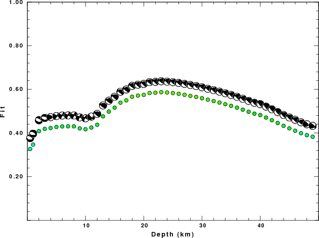
The best solution is
WVFGRD96 23.0 245 35 30 5.07 0.5871
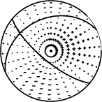
The mechanism correspond to the best fit is
|
|
|
The best fit as a function of depth is given in the following figure:
|
|
|
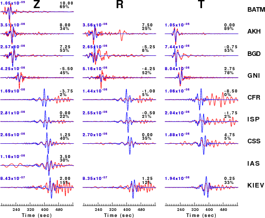
The comparison of the observed and predicted waveforms is given in the next figure. The red traces are the observed and the blue are the predicted. Each observed-predicted component is plotted to the same scale and peak amplitudes are indicated by the numbers to the left of each trace. A pair of numbers is given in black at the right of each predicted traces. The upper number it the time shift required for maximum correlation between the observed and predicted traces. This time shift is required because the synthetics are not computed at exactly the same distance as the observed and because the velocity model used in the predictions may not be perfect. A positive time shift indicates that the prediction is too fast and should be delayed to match the observed trace (shift to the right in this figure). A negative value indicates that the prediction is too slow. The lower number gives the percentage of variance reduction to characterize the individual goodness of fit (100% indicates a perfect fit).
The bandpass filter used in the processing and for the display was
hp c 0.02 n 3
lp c 0.05 n 3
|
|
|
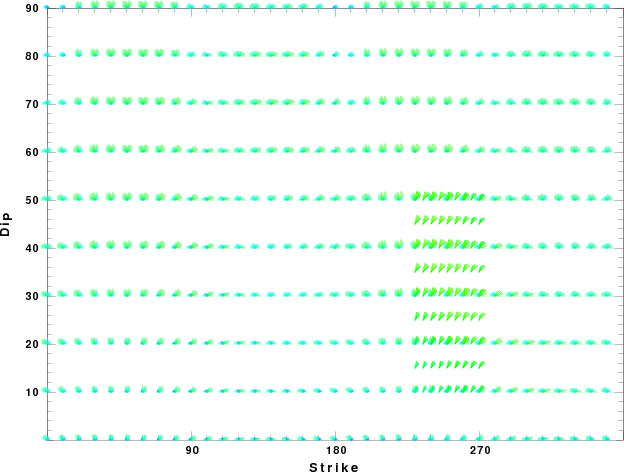
|
| Focal mechanism sensitivity at the preferred depth. The red color indicates a very good fit to thewavefroms. Each solution is plotted as a vector at a given value of strike and dip with the angle of the vector representing the rake angle, measured, with respect to the upward vertical (N) in the figure. |
A check on the assumed source location is possible by looking at the time shifts between the observed and predicted traces. The time shifts for waveform matching arise for several reasons:
Time_shift = A + B cos Azimuth + C Sin Azimuth
The time shifts for this inversion lead to the next figure:
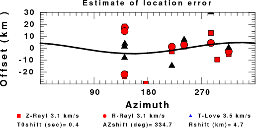
The derived shift in origin time and epicentral coordinates are given at the bottom of the figure.
Should the national backbone of the USGS Advanced National Seismic System (ANSS) be implemented with an interstation separation of 300 km, it is very likely that an earthquake such as this would have been recorded at distances on the order of 100-200 km. This means that the closest station would have information on source depth and mechanism that was lacking here.
Dr. Harley Benz, USGS, provided the USGS USNSN digital data. The digital data used in this study were provided by Natural Resources Canada through their AUTODRM site http://www.seismo.nrcan.gc.ca/nwfa/autodrm/autodrm_req_e.php, and IRIS using their BUD interface.
Thanks also to the many seismic network operators whose dedication make this effort possible: University of Alaska, University of Washington, Oregon State University, University of Utah, Montana Bureas of Mines, UC Berkely, Caltech, UC San Diego, Saint L ouis University, Universityof Memphis, Lamont Doehrty Earth Observatory, Boston College, the Iris stations and the Transportable Array of EarthScope.
The WUS used for the waveform synthetic seismograms and for the surface wave eigenfunctions and dispersion is as follows:
MODEL.01
Model after     8 iterations
ISOTROPIC
KGS
FLAT EARTH
1-D
CONSTANT VELOCITY
LINE08
LINE09
LINE10
LINE11
      H(KM)   VP(KM/S)   VS(KM/S) RHO(GM/CC)         QP         QS       ETAP       ETAS      FREFP      FREFS
     1.9000     3.4065     2.0089     2.2150  0.302E-02  0.679E-02   0.00       0.00       1.00       1.00
     6.1000     5.5445     3.2953     2.6089  0.349E-02  0.784E-02   0.00       0.00       1.00       1.00
    13.0000     6.2708     3.7396     2.7812  0.212E-02  0.476E-02   0.00       0.00       1.00       1.00
    19.0000     6.4075     3.7680     2.8223  0.111E-02  0.249E-02   0.00       0.00       1.00       1.00
     0.0000     7.9000     4.6200     3.2760  0.164E-10  0.370E-10   0.00       0.00       1.00       1.00
Here we tabulate the reasons for not using certain digital data sets
The following stations did not have a valid response files:
DATE=Thu Jun 20 03:46:14 CDT 2013