THE SLU location for this event is 2010/09/15 02:23:13 45.59 14.25 15.7 Slovenia
We read arrival times from waveforms downloaded from EIDA and picked first motions. We used both the nnCIA and WUS velocity models. The nnCIA model gave a shallow depth than the WUS model. However we prefer the use of the WUS model because of the waveforms fits. The output of the elocate computations is in the file elocate.txt.
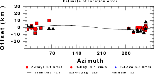
As a test on the SLU solution, we examined the azimuthal distribution of time shifts required for the waveform match. These were fit to an equaiton of the form
TimeShift = A + B sin Az + C cos Az
The B and C terms are related to a spatial shift of the epicenter DR through the assumed group velocity of the Love and Rayleigh waves, which we take to be 3.1/0.92 and 3.1 km/s respectively. The next figure shows the pattern of inferred residuals in distance to each station.
The simplified analysis calls for the origin time to be 0.6 sec earlier than the SLU soltuion and for the SLU epicenter to move about 3 km to the east. These are not significant shifts. The SLU solution is accepted.
 USGS/SLU Moment Tensor Solution
 ENS  2010/09/15 02:23:13:0  45.59   14.25  15.7 0.0 Slovenia

 Best Fitting Double Couple
  Mo = 4.47e+21 dyne-cm
  Mw = 3.70
  Z  = 25 km
  Plane   Strike  Dip  Rake
   NP1      250    80    15
   NP2      157    75   170
  Principal Axes:
   Axis    Value   Plunge  Azimuth
    T   4.47e+21     18     114
    N   0.00e+00     72     283
    P  -4.47e+21      3      23

 Moment Tensor: (dyne-cm)
    Component   Value
       Mxx    -3.08e+21
       Mxy    -3.13e+21
       Mxz    -7.65e+20
       Myy     2.69e+21
       Myz     1.08e+21
       Mzz     3.95e+20


                     -------------
                 ###-------------- P --
              ######--------------   -----
             #######-----------------------
           #########-------------------------
          ###########-------------------------
         ############--------------------------
        ##############--------------------######
        ##############------------##############
       ################-----#####################
       ################-#########################
       ############-----#########################
       ########----------########################
        ####--------------################   ###
        #------------------############### T ###
         -------------------##############   ##
          -------------------#################
           -------------------###############
             ------------------############
              -------------------#########
                 -----------------#####
                     --------------


 Global CMT Convention Moment Tensor:
      R          T          P
  3.95e+20  -7.65e+20  -1.08e+21
 -7.65e+20  -3.08e+21   3.13e+21
 -1.08e+21   3.13e+21   2.69e+21


Details of the solution is found at

http://www.eas.slu.edu/Earthquake_Center/MECH.NA/20100915022313/index.html
|
      STK = 250
      DIP = 80
     RAKE = 15
       MW = 3.70
       HS = 25.0
The waveform inversion is preferred.
The following compares this source inversion to others
 USGS/SLU Moment Tensor Solution
 ENS  2010/09/15 02:21:17:0  45.62   14.26   2.0 3.8 Slovenia

 Best Fitting Double Couple
  Mo = 8.61e+21 dyne-cm
  Mw = 3.89
  Z  = 25 km
  Plane   Strike  Dip  Rake
   NP1      156    81   155
   NP2      250    65    10
  Principal Axes:
   Axis    Value   Plunge  Azimuth
    T   8.61e+21     24     110
    N   0.00e+00     63     317
    P  -8.61e+21     11     205

 Moment Tensor: (dyne-cm)
    Component   Value
       Mxx    -5.95e+21
       Mxy    -5.52e+21
       Mxz     3.23e+20
       Myy     4.81e+21
       Myz     3.70e+21
       Mzz     1.15e+21


                     --------------
                 ###-------------------
              ######----------------------
             #######-----------------------
           ##########------------------------
          ############------------------------
         #############--------------#######----
        ###############----#####################
        ###############-########################
       ############-----#########################
       #########---------########################
       #######------------#######################
       #####---------------######################
        ##------------------#############   ####
        #--------------------############ T ####
         ---------------------###########   ###
          ---------------------###############
           ---------------------#############
             --------------------##########
              -----   ------------########
                 -- P -------------####
                      -------------


 Global CMT Convention Moment Tensor:
      R          T          P
  1.15e+21   3.23e+20  -3.70e+21
  3.23e+20  -5.95e+21   5.52e+21
 -3.70e+21   5.52e+21   4.81e+21


Details of the solution is found at

http://www.eas.slu.edu/Earthquake_Center/MECH.NA/20100915022117/index.html
 USGS/SLU Moment Tensor Solution
 ENS  2010/09/15 02:23:13:0  45.59   14.25  15.7 0.0 Slovenia

 Best Fitting Double Couple
  Mo = 4.47e+21 dyne-cm
  Mw = 3.70
  Z  = 25 km
  Plane   Strike  Dip  Rake
   NP1      250    80    15
   NP2      157    75   170
  Principal Axes:
   Axis    Value   Plunge  Azimuth
    T   4.47e+21     18     114
    N   0.00e+00     72     283
    P  -4.47e+21      3      23

 Moment Tensor: (dyne-cm)
    Component   Value
       Mxx    -3.08e+21
       Mxy    -3.13e+21
       Mxz    -7.65e+20
       Myy     2.69e+21
       Myz     1.08e+21
       Mzz     3.95e+20


                     -------------
                 ###-------------- P --
              ######--------------   -----
             #######-----------------------
           #########-------------------------
          ###########-------------------------
         ############--------------------------
        ##############--------------------######
        ##############------------##############
       ################-----#####################
       ################-#########################
       ############-----#########################
       ########----------########################
        ####--------------################   ###
        #------------------############### T ###
         -------------------##############   ##
          -------------------#################
           -------------------###############
             ------------------############
              -------------------#########
                 -----------------#####
                     --------------


 Global CMT Convention Moment Tensor:
      R          T          P
  3.95e+20  -7.65e+20  -1.08e+21
 -7.65e+20  -3.08e+21   3.13e+21
 -1.08e+21   3.13e+21   2.69e+21


Details of the solution is found at

http://www.eas.slu.edu/Earthquake_Center/MECH.NA/20100915022313/index.html
|
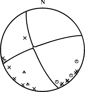
First motion solution using the polarity picks, azimuths and takeoff angles indicated in the elocate.txt output. The nodal planes plotted are those of the preferred solution. |
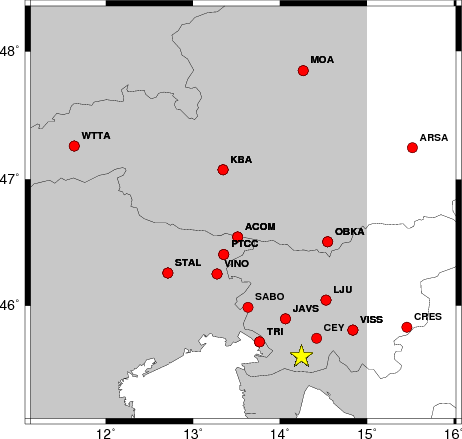
The focal mechanism was determined using broadband seismic waveforms. The location of the event and the and stations used for the waveform inversion are shown in the next figure.
|
|
|
The program wvfgrd96 was used with good traces observed at short distance to determine the focal mechanism, depth and seismic moment. This technique requires a high quality signal and well determined velocity model for the Green functions. To the extent that these are the quality data, this type of mechanism should be preferred over the radiation pattern technique which requires the separate step of defining the pressure and tension quadrants and the correct strike.
The observed and predicted traces are filtered using the following gsac commands:
hp c 0.02 n 3
lp c 0.10 n 3
The results of this grid search from 0.5 to 19 km depth are as follow:
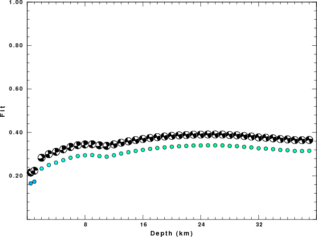
           DEPTH  STK   DIP  RAKE   MW    FIT
WVFGRD96    0.5   130    50   -65   3.12 0.1658
WVFGRD96    1.0   165    90    -5   3.06 0.1737
WVFGRD96    2.0   335    60   -25   3.25 0.2338
WVFGRD96    3.0   345    90     5   3.27 0.2502
WVFGRD96    4.0   165    75    15   3.33 0.2610
WVFGRD96    5.0   165    70    15   3.37 0.2726
WVFGRD96    6.0   165    70    15   3.40 0.2834
WVFGRD96    7.0   165    75    15   3.43 0.2913
WVFGRD96    8.0   165    70    15   3.48 0.2950
WVFGRD96    9.0   165    70    15   3.50 0.2958
WVFGRD96   10.0   340    80   -25   3.53 0.2910
WVFGRD96   11.0   340    75   -15   3.54 0.2884
WVFGRD96   12.0   255    85    15   3.55 0.2952
WVFGRD96   13.0   255    85    15   3.57 0.3029
WVFGRD96   14.0   250    85    15   3.58 0.3092
WVFGRD96   15.0   250    85    15   3.59 0.3148
WVFGRD96   16.0   250    85    15   3.61 0.3199
WVFGRD96   17.0   250    80    15   3.62 0.3245
WVFGRD96   18.0   250    80    15   3.63 0.3284
WVFGRD96   19.0   250    80    15   3.64 0.3313
WVFGRD96   20.0   250    80    10   3.66 0.3343
WVFGRD96   21.0   250    80    15   3.67 0.3365
WVFGRD96   22.0   250    80    15   3.67 0.3380
WVFGRD96   23.0   250    80    15   3.68 0.3399
WVFGRD96   24.0   250    80    15   3.69 0.3400
WVFGRD96   25.0   250    80    15   3.70 0.3408
WVFGRD96   26.0   250    80    15   3.71 0.3407
WVFGRD96   27.0   250    80    15   3.71 0.3404
WVFGRD96   28.0   250    75    15   3.72 0.3380
WVFGRD96   29.0   250    75    15   3.72 0.3369
WVFGRD96   30.0   250    75    15   3.73 0.3337
WVFGRD96   31.0   250    75    10   3.73 0.3311
WVFGRD96   32.0   255    75     0   3.74 0.3271
WVFGRD96   33.0   255    75     0   3.75 0.3256
WVFGRD96   34.0   255    75     0   3.75 0.3230
WVFGRD96   35.0   255    75     0   3.76 0.3197
WVFGRD96   36.0   255    75     0   3.77 0.3181
WVFGRD96   37.0   255    75     0   3.78 0.3148
WVFGRD96   38.0   255    75     0   3.79 0.3145
WVFGRD96   39.0   255    80     0   3.82 0.3155
The best solution is
WVFGRD96 25.0 250 80 15 3.70 0.3408
The mechanism correspond to the best fit is
|
|
|
The best fit as a function of depth is given in the following figure:
|
|
|
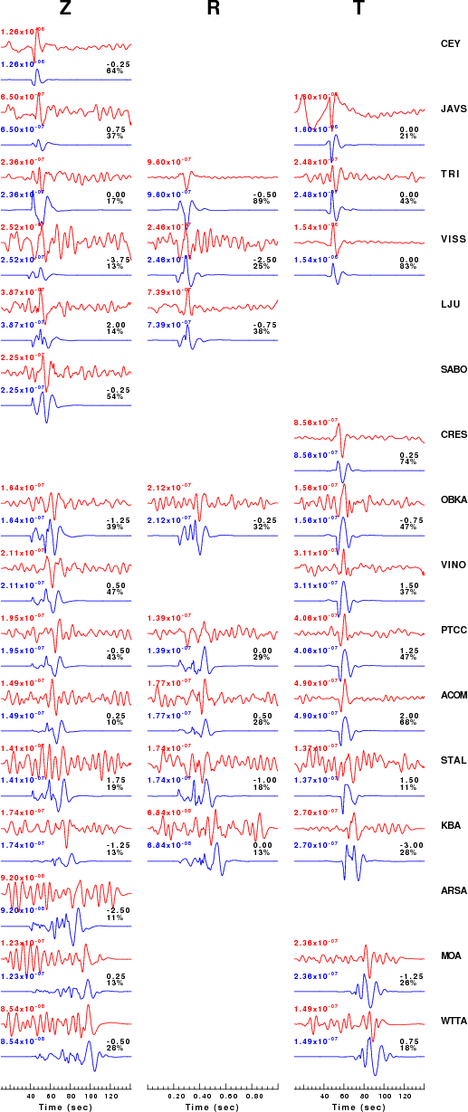
The comparison of the observed and predicted waveforms is given in the next figure. The red traces are the observed and the blue are the predicted. Each observed-predicted componnet is plotted to the same scale and peak amplitudes are indicated by the numbers to the left of each trace. The number in black at the rightr of each predicted traces it the time shift required for maximum correlation between the observed and predicted traces. This time shift is required because the synthetics are not computed at exactly the same distance as the observed and because the velocity model used in the predictions may not be perfect. A positive time shift indicates that the prediction is too fast and should be delayed to match the observed trace (shift to the right in this figure). A negative value indicates that the prediction is too slow. The bandpass filter used in the processing and for the display was
hp c 0.02 n 3
lp c 0.10 n 3
|
|
|
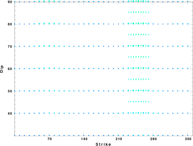
|
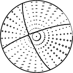
| Focal mechanism sensitivity at the preferred depth. The red color indicates a very good fit to thewavefroms. Each solution is plotted as a vector at a given value of strike and dip with the angle of the vector representing the rake angle, measured, with respect to the upward vertical (N) in the figure. |
The WUS used for the waveform synthetic seismograms and for the surface wave eigenfunctions and dispersion is as follows:
MODEL.01
Model after     8 iterations
ISOTROPIC
KGS
FLAT EARTH
1-D
CONSTANT VELOCITY
LINE08
LINE09
LINE10
LINE11
      H(KM)   VP(KM/S)   VS(KM/S) RHO(GM/CC)         QP         QS       ETAP       ETAS      FREFP      FREFS
     1.9000     3.4065     2.0089     2.2150  0.302E-02  0.679E-02   0.00       0.00       1.00       1.00
     6.1000     5.5445     3.2953     2.6089  0.349E-02  0.784E-02   0.00       0.00       1.00       1.00
    13.0000     6.2708     3.7396     2.7812  0.212E-02  0.476E-02   0.00       0.00       1.00       1.00
    19.0000     6.4075     3.7680     2.8223  0.111E-02  0.249E-02   0.00       0.00       1.00       1.00
     0.0000     7.9000     4.6200     3.2760  0.164E-10  0.370E-10   0.00       0.00       1.00       1.00
Here we tabulate the reasons for not using certain digital data sets
The following stations did not have a valid response files:
DATE=Wed Sep 15 15:11:02 CDT 2010