2008/09/06 19:48:03 45.8560 26.4780 31.0 4.70 ROMANIA
USGS Felt map for this earthquake
 USGS/SLU Moment Tensor Solution
 2008/09/06 19:48:03  45.8560  26.4780  31.0  4.70 ROMANIA

 Best Fitting Double Couple
    Mo = 2.09e+22 dyne-cm
    Mw = 4.18
    Z  = 14 km
     Plane   Strike  Dip  Rake
      NP1      337    80   107
      NP2       95    20    30
 Principal Axes:
   Axis    Value   Plunge  Azimuth
     T   2.09e+22     52     267
     N   0.00e+00     17     153
     P  -2.09e+22     33      52


 Moment Tensor: (dyne-cm)
    Component  Value
       Mxx    -5.59e+21
       Mxy    -6.68e+21
       Mxz    -6.49e+21
       Myy    -1.13e+21
       Myz    -1.76e+22
       Mzz     6.71e+21


                     --------------
                 ####------------------
              ########--------------------
             ###########-------------------
           ##############--------------------
          ################------------   -----
         ##################----------- P ------
        ####################----------   -------
        #####################-------------------
       #######################-------------------
       ##########   ##########-------------------
       -######### T ###########------------------
       -#########   ############----------------#
        -########################---------------
        --#######################--------------#
         --#######################------------#
          ---#####################----------##
           ----####################-------###
             ----##################----####
              -------##############-######
                 -------------------###
                     --------------


 Harvard Convention
 Moment Tensor:
      R          T          F
  6.71e+21  -6.49e+21   1.76e+22
 -6.49e+21  -5.59e+21   6.68e+21
  1.76e+22   6.68e+21  -1.13e+21


Details of the solution is found at

http://www.eas.slu.edu/Earthquake_Center/MECH.NA/20080906194803/index.html
|
      STK = 95
      DIP = 20
     RAKE = 30
       MW = 4.18
       HS = 14.0
The waveform inversion is preferred.
The following compares this source inversion to others
 USGS/SLU Moment Tensor Solution
 2008/09/06 19:48:03  45.8560  26.4780  31.0  4.70 ROMANIA

 Best Fitting Double Couple
    Mo = 2.09e+22 dyne-cm
    Mw = 4.18
    Z  = 14 km
     Plane   Strike  Dip  Rake
      NP1      337    80   107
      NP2       95    20    30
 Principal Axes:
   Axis    Value   Plunge  Azimuth
     T   2.09e+22     52     267
     N   0.00e+00     17     153
     P  -2.09e+22     33      52


 Moment Tensor: (dyne-cm)
    Component  Value
       Mxx    -5.59e+21
       Mxy    -6.68e+21
       Mxz    -6.49e+21
       Myy    -1.13e+21
       Myz    -1.76e+22
       Mzz     6.71e+21


                     --------------
                 ####------------------
              ########--------------------
             ###########-------------------
           ##############--------------------
          ################------------   -----
         ##################----------- P ------
        ####################----------   -------
        #####################-------------------
       #######################-------------------
       ##########   ##########-------------------
       -######### T ###########------------------
       -#########   ############----------------#
        -########################---------------
        --#######################--------------#
         --#######################------------#
          ---#####################----------##
           ----####################-------###
             ----##################----####
              -------##############-######
                 -------------------###
                     --------------


 Harvard Convention
 Moment Tensor:
      R          T          F
  6.71e+21  -6.49e+21   1.76e+22
 -6.49e+21  -5.59e+21   6.68e+21
  1.76e+22   6.68e+21  -1.13e+21


Details of the solution is found at

http://www.eas.slu.edu/Earthquake_Center/MECH.NA/20080906194803/index.html
|
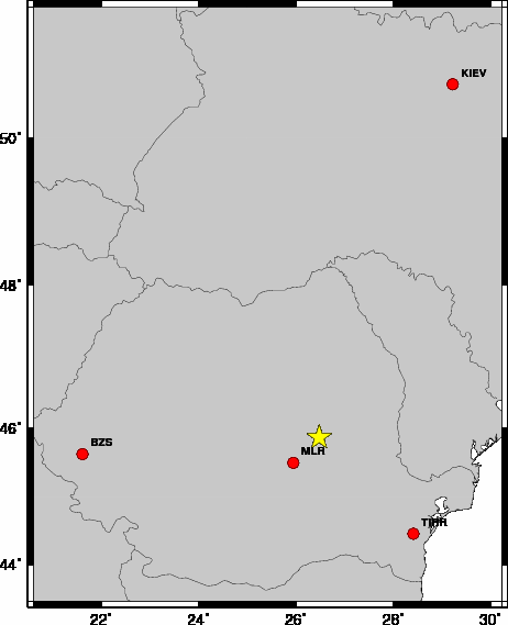
The focal mechanism was determined using broadband seismic waveforms. The location of the event and the and stations used for the waveform inversion are shown in the next figure.
|
|
|
|
The program wvfgrd96 was used with good traces observed at short distance to determine the focal mechanism, depth and seismic moment. This technique requires a high quality signal and well determined velocity model for the Green functions. To the extent that these are the quality data, this type of mechanism should be preferred over the radiation pattern technique which requires the separate step of defining the pressure and tension quadrants and the correct strike.
The observed and predicted traces are filtered using the following gsac commands:
hp c 0.02 n 3
lp c 0.05 n 3
The results of this grid search from 0.5 to 19 km depth are as follow:
           DEPTH  STK   DIP  RAKE   MW    FIT
WVFGRD96    0.5    95    60    30   3.88 0.3367
WVFGRD96    1.0    90    75    15   3.91 0.3360
WVFGRD96    2.0    95    65    30   3.99 0.3693
WVFGRD96    3.0    90    65   -15   4.07 0.3649
WVFGRD96    4.0    80     5    15   4.16 0.4298
WVFGRD96    5.0    75    10     5   4.16 0.5424
WVFGRD96    6.0    80    10    15   4.15 0.6199
WVFGRD96    7.0    85    10    20   4.14 0.6736
WVFGRD96    8.0    85    10    20   4.21 0.7088
WVFGRD96    9.0    85    10    20   4.20 0.7424
WVFGRD96   10.0    95    15    30   4.19 0.7649
WVFGRD96   11.0    95    15    30   4.19 0.7808
WVFGRD96   12.0    95    15    30   4.18 0.7880
WVFGRD96   13.0    95    20    30   4.18 0.7913
WVFGRD96   14.0    95    20    30   4.18 0.7914
WVFGRD96   15.0   105    20    50   4.17 0.7885
WVFGRD96   16.0   105    20    50   4.17 0.7840
WVFGRD96   17.0   295    75    85   4.18 0.7785
WVFGRD96   18.0   125    20    95   4.18 0.7700
WVFGRD96   19.0   125    20    95   4.18 0.7619
WVFGRD96   20.0   300    70    90   4.18 0.7508
WVFGRD96   21.0   120    15    95   4.19 0.7412
WVFGRD96   22.0   120    15    95   4.19 0.7292
WVFGRD96   23.0   120    15    95   4.19 0.7168
WVFGRD96   24.0   115    15    90   4.20 0.7047
WVFGRD96   25.0   110    15    85   4.20 0.6919
WVFGRD96   26.0   110    15    85   4.20 0.6794
WVFGRD96   27.0   110    15    85   4.20 0.6668
WVFGRD96   28.0   110    15    85   4.20 0.6538
WVFGRD96   29.0   110    15    80   4.20 0.6407
WVFGRD96   30.0   100    15    70   4.20 0.6281
WVFGRD96   31.0   105    15    75   4.20 0.6162
WVFGRD96   32.0   105    15    75   4.21 0.6038
WVFGRD96   33.0   110    15    80   4.21 0.5913
WVFGRD96   34.0   100    15    70   4.21 0.5802
WVFGRD96   35.0    85    70    25   4.37 0.5701
WVFGRD96   36.0    85    70    20   4.37 0.5691
WVFGRD96   37.0    85    70    20   4.39 0.5674
WVFGRD96   38.0    85    75    15   4.41 0.5637
WVFGRD96   39.0    85    75    15   4.43 0.5589
WVFGRD96   40.0    90    60    30   4.46 0.5623
WVFGRD96   41.0    90    60    30   4.47 0.5560
WVFGRD96   42.0    90    60    25   4.47 0.5501
WVFGRD96   43.0    85    70    20   4.49 0.5442
WVFGRD96   44.0    85    65    20   4.48 0.5379
WVFGRD96   45.0    85    65    20   4.49 0.5321
WVFGRD96   46.0    85    65    20   4.50 0.5272
WVFGRD96   47.0    85    65    20   4.50 0.5212
WVFGRD96   48.0    85    65    20   4.51 0.5152
WVFGRD96   49.0    85    65    20   4.52 0.5092
WVFGRD96   50.0    85    65    20   4.52 0.5027
The best solution is
WVFGRD96 14.0 95 20 30 4.18 0.7914
The mechanism correspond to the best fit is
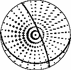
|
|
|
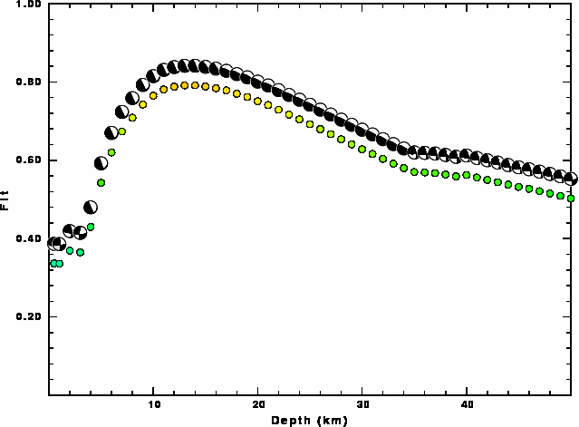
The best fit as a function of depth is given in the following figure:
|
|
|
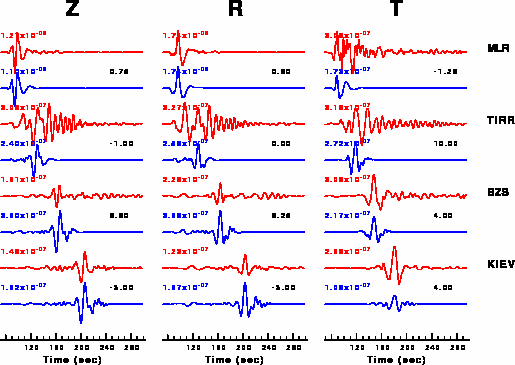
The comparison of the observed and predicted waveforms is given in the next figure. The red traces are the observed and the blue are the predicted. Each observed-predicted componnet is plotted to the same scale and peak amplitudes are indicated by the numbers to the left of each trace. The number in black at the rightr of each predicted traces it the time shift required for maximum correlation between the observed and predicted traces. This time shift is required because the synthetics are not computed at exactly the same distance as the observed and because the velocity model used in the predictions may not be perfect. A positive time shift indicates that the prediction is too fast and should be delayed to match the observed trace (shift to the right in this figure). A negative value indicates that the prediction is too slow. The bandpass filter used in the processing and for the display was
hp c 0.02 n 3
lp c 0.05 n 3
|
|
|
|
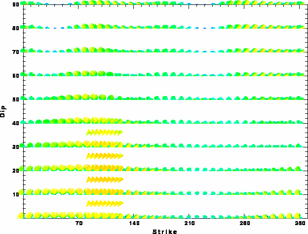
| Focal mechanism sensitivity at the preferred depth. The red color indicates a very good fit to thewavefroms. Each solution is plotted as a vector at a given value of strike and dip with the angle of the vector representing the rake angle, measured, with respect to the upward vertical (N) in the figure. |
Should the national backbone of the USGS Advanced National Seismic System (ANSS) be implemented with an interstation separation of 300 km, it is very likely that an earthquake such as this would have been recorded at distances on the order of 100-200 km. This means that the closest station would have information on source depth and mechanism that was lacking here.
Dr. Harley Benz, USGS, provided the USGS USNSN digital data. The digital data used in this study were provided by Natural Resources Canada through their AUTODRM site http://www.seismo.nrcan.gc.ca/nwfa/autodrm/autodrm_req_e.php, and IRIS using their BUD interface.
Thanks also to the many seismic network operators whose dedication make this effort possible: University of Alaska, University of Washington, Oregon State University, University of Utah, Montana Bureas of Mines, UC Berkely, Caltech, UC San Diego, Saint L ouis University, Universityof Memphis, Lamont Doehrty Earth Observatory, Boston College, the Iris stations and the Transportable Array of EarthScope.
The WUS used for the waveform synthetic seismograms and for the surface wave eigenfunctions and dispersion is as follows:
MODEL.01
Model after     8 iterations
ISOTROPIC
KGS
FLAT EARTH
1-D
CONSTANT VELOCITY
LINE08
LINE09
LINE10
LINE11
      H(KM)   VP(KM/S)   VS(KM/S) RHO(GM/CC)         QP         QS       ETAP       ETAS      FREFP      FREFS
     1.9000     3.4065     2.0089     2.2150  0.302E-02  0.679E-02   0.00       0.00       1.00       1.00
     6.1000     5.5445     3.2953     2.6089  0.349E-02  0.784E-02   0.00       0.00       1.00       1.00
    13.0000     6.2708     3.7396     2.7812  0.212E-02  0.476E-02   0.00       0.00       1.00       1.00
    19.0000     6.4075     3.7680     2.8223  0.111E-02  0.249E-02   0.00       0.00       1.00       1.00
     0.0000     7.9000     4.6200     3.2760  0.164E-10  0.370E-10   0.00       0.00       1.00       1.00
Here we tabulate the reasons for not using certain digital data sets
The following stations did not have a valid response files:
DATE=Sat Sep 6 16:14:45 MDT 2008