2008/02/27 00:56:45 53.32 -0.31 10.0 4.7 England USGS
2008/02/27 00:56:43.9 53.3357 -0.4281 2.0 4.9 EMSC
USGS Felt map for this earthquake
 SLU Moment Tensor Solution
 2008/02/27 00:56:45 53.32 -0.31 10.0 4.7 England

 Best Fitting Double Couple
    Mo = 6.17e+22 dyne-cm
    Mw = 4.46
    Z  = 25 km
     Plane   Strike  Dip  Rake
      NP1       97    86   145
      NP2      190    55     5
 Principal Axes:
   Axis    Value   Plunge  Azimuth
     T   6.17e+22     27      48
     N   0.00e+00     55     271
     P  -6.17e+22     21     149


 Moment Tensor: (dyne-cm)
    Component  Value
       Mxx    -1.74e+22
       Mxy     4.81e+22
       Mxz     3.44e+22
       Myy     1.23e+22
       Myz     7.93e+21
       Mzz     5.05e+21


                     ---------#####
                 ----------############
              ------------################
             -----------###################
           ------------###############   ####
          ------------################ T #####
         ------------#################   ######
        -------------###########################
        ------------############################
       -------------#############################
       ########----##############################
       ############--------######################
       ############------------------------------
        ###########-----------------------------
        ###########-----------------------------
         ##########----------------------------
          #########---------------------------
           #########---------------   -------
             #######--------------- P -----
              #######--------------   ----
                 #####-----------------
                     ##------------


 Harvard Convention
 Moment Tensor:
      R          T          F
  5.05e+21   3.44e+22  -7.93e+21
  3.44e+22  -1.74e+22  -4.81e+22
 -7.93e+21  -4.81e+22   1.23e+22


Details of the solution is found at

http://www.eas.slu.edu/Earthquake_Center/MECH.NA/20080227005645/index.html
|
      STK = 190
      DIP = 55
     RAKE = 5
       MW = 4.46
       HS = 25
The wavefrom inversion solution is preferred.
The following compares this source inversion to others
 SLU Moment Tensor Solution
 2008/02/27 00:56:45 53.32 -0.31 10.0 4.7 England

 Best Fitting Double Couple
    Mo = 6.17e+22 dyne-cm
    Mw = 4.46
    Z  = 25 km
     Plane   Strike  Dip  Rake
      NP1       97    86   145
      NP2      190    55     5
 Principal Axes:
   Axis    Value   Plunge  Azimuth
     T   6.17e+22     27      48
     N   0.00e+00     55     271
     P  -6.17e+22     21     149


 Moment Tensor: (dyne-cm)
    Component  Value
       Mxx    -1.74e+22
       Mxy     4.81e+22
       Mxz     3.44e+22
       Myy     1.23e+22
       Myz     7.93e+21
       Mzz     5.05e+21


                     ---------#####
                 ----------############
              ------------################
             -----------###################
           ------------###############   ####
          ------------################ T #####
         ------------#################   ######
        -------------###########################
        ------------############################
       -------------#############################
       ########----##############################
       ############--------######################
       ############------------------------------
        ###########-----------------------------
        ###########-----------------------------
         ##########----------------------------
          #########---------------------------
           #########---------------   -------
             #######--------------- P -----
              #######--------------   ----
                 #####-----------------
                     ##------------


 Harvard Convention
 Moment Tensor:
      R          T          F
  5.05e+21   3.44e+22  -7.93e+21
  3.44e+22  -1.74e+22  -4.81e+22
 -7.93e+21  -4.81e+22   1.23e+22


Details of the solution is found at

http://www.eas.slu.edu/Earthquake_Center/MECH.NA/20080227005645/index.html
|
EMSC Moment Tensors solutions

Provided by ETHZ, AUTH, IGN, INGV-MEDNET, KOERI, NOA_IG, HARVARD, USGS, CPPT

From: pondrix@bo.ingv.it
FID: AUX18
DAT: 200802271502 GMT

S022708A 02/27/08 00:56:43.9  53.34   -0.43  10.04.90.0UNITED KINGDOM  MW=4.63
Nei BW: 0  0   0 SW:26 41  35 DT=   3.5 1.0  53.39 0.02   -0.41 0.08  25.2  1.3
 DUR 0.5 EX 23  0.04 0.09 -0.41 0.06  0.37 0.05  0.38 0.07 -0.22 0.07 -0.93 0.05
   1.13 20  55  -0.07 67 265  -1.06 11 149   1.10 193 68    7 100 83  158
CENTROID, MOMENT TENSOR SOLUTION
HARVARD EVENT-FILE NAME S022708A
DATA USED: GSN
SURFACE WAVES:   26S, 41C, T= 35
CENTROID LOCATION:
ORIGIN TIME       00:56:47.4 1.0
LAT 53.39N 0.02;LON   0.41W 0.08
DEP  25.2 1.3;HALF-DURATION  0.5
MOMENT TENSOR; SCALE 10**23 D-CM
  MRR= 0.04 0.09; MTT=-0.41 0.06
  MPP= 0.37 0.05; MRT= 0.38 0.07
  MRP=-0.22 0.07; MTP=-0.93 0.05
 PRINCIPAL AXES:
 1.(T) VAL=  1.13;PLG=20;AZM= 55
 2.(N)      -0.07;    67;    265
 3.(P)      -1.06;    11;    149
BEST DOUBLE COUPLE:M0=1.1*10**23
 NP1:STRIKE=193;DIP=68;SLIP=   7
 NP2:STRIKE=100;DIP=83;SLIP= 158

            ---------##
        -----------########
      ------------###########
    ------------###########   #
   -------------########### T ##
  -------------############   ###
  ------------###################
 #------------####################
 ######------#####################
 ############--###################
 ###########----------------######
  ##########---------------------
  ##########---------------------
   #########--------------------
    ########------------   ----
      ######------------ P --
        #####-----------
            ##---------
|
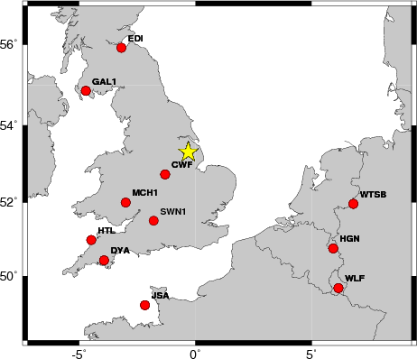
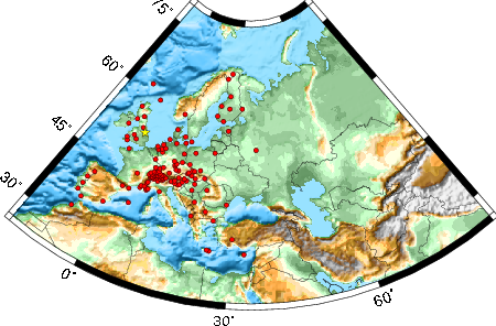
The focal mechanism was determined using broadband seismic waveforms. The location of the event and the and stations used for the waveform inversion are shown in the next figure.
|
|
|
|
The program wvfgrd96 was used with good traces observed at short distance to determine the focal mechanism, depth and seismic moment. This technique requires a high quality signal and well determined velocity model for the Green functions. To the extent that these are the quality data, this type of mechanism should be preferred over the radiation pattern technique which requires the separate step of defining the pressure and tension quadrants and the correct strike.
The observed and predicted traces are filtered using the following gsac commands:
hp c 0.02 n 3
lp c 0.05 n 3
The results of this grid search from 0.5 to 19 km depth are as follow:
           DEPTH  STK   DIP  RAKE   MW    FIT
WVFGRD96    0.5   110    50    85   3.96 0.2339
WVFGRD96    1.0   185    90    -5   4.02 0.2358
WVFGRD96    2.0     5    80   -10   4.12 0.2869
WVFGRD96    3.0     5    90     0   4.18 0.3090
WVFGRD96    4.0   185    85    -5   4.23 0.3129
WVFGRD96    5.0   195    60    30   4.30 0.3282
WVFGRD96    6.0   195    55    30   4.32 0.3646
WVFGRD96    7.0   195    55    25   4.32 0.3937
WVFGRD96    8.0   200    50    35   4.39 0.4279
WVFGRD96    9.0   195    50    25   4.39 0.4559
WVFGRD96   10.0   195    70    45   4.41 0.4898
WVFGRD96   11.0   200    60    40   4.41 0.5199
WVFGRD96   12.0   195    65    35   4.41 0.5490
WVFGRD96   13.0   195    60    30   4.41 0.5745
WVFGRD96   14.0   195    60    30   4.42 0.5965
WVFGRD96   15.0   195    60    25   4.42 0.6140
WVFGRD96   16.0   195    60    25   4.42 0.6303
WVFGRD96   17.0   195    60    25   4.43 0.6432
WVFGRD96   18.0   190    60    15   4.44 0.6550
WVFGRD96   19.0   190    60    15   4.44 0.6645
WVFGRD96   20.0   190    60    10   4.45 0.6717
WVFGRD96   21.0   190    55    10   4.45 0.6779
WVFGRD96   22.0   190    55    10   4.45 0.6820
WVFGRD96   23.0   190    55    10   4.45 0.6843
WVFGRD96   24.0   190    55    10   4.46 0.6852
WVFGRD96   25.0   190    55     5   4.46 0.6852
WVFGRD96   26.0   190    55     5   4.46 0.6840
WVFGRD96   27.0   190    55     5   4.46 0.6818
WVFGRD96   28.0   190    55     5   4.47 0.6786
WVFGRD96   29.0   190    55     5   4.47 0.6744
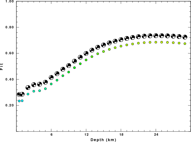
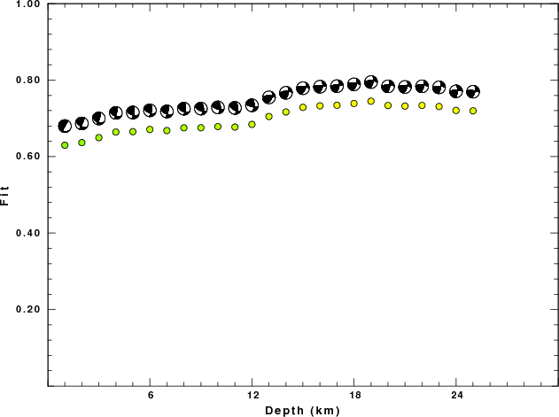
The best solution is
WVFGRD96 25.0 190 55 5 4.46 0.6852
The mechanism correspond to the best fit is
|
|
|
The best fit as a function of depth is given in the following figure:
|
|
|
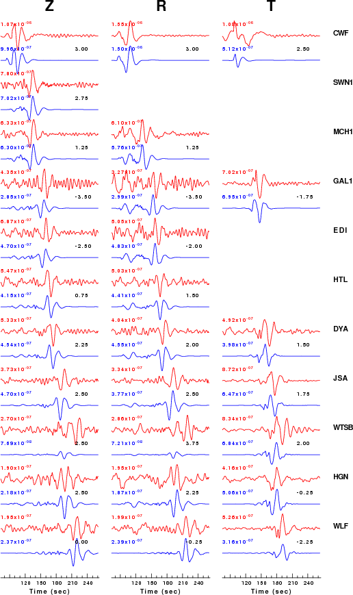
The comparison of the observed and predicted waveforms is given in the next figure. The red traces are the observed and the blue are the predicted. Each observed-predicted componnet is plotted to the same scale and peak amplitudes are indicated by the numbers to the left of each trace. The number in black at the rightr of each predicted traces it the time shift required for maximum correlation between the observed and predicted traces. This time shift is required because the synthetics are not computed at exactly the same distance as the observed and because the velocity model used in the predictions may not be perfect. A positive time shift indicates that the prediction is too fast and should be delayed to match the observed trace (shift to the right in this figure). A negative value indicates that the prediction is too slow. The bandpass filter used in the processing and for the display was
hp c 0.02 n 3
lp c 0.05 n 3
|
|
|
|
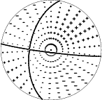
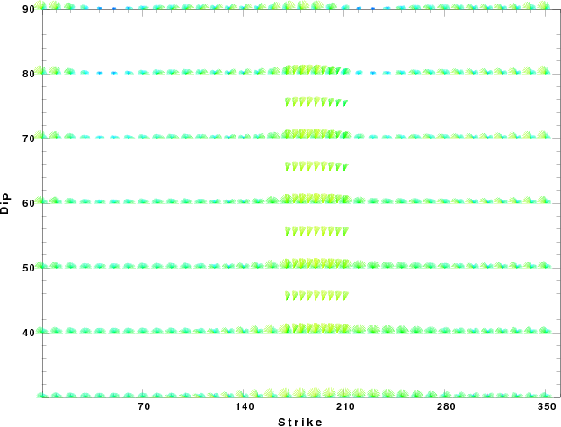
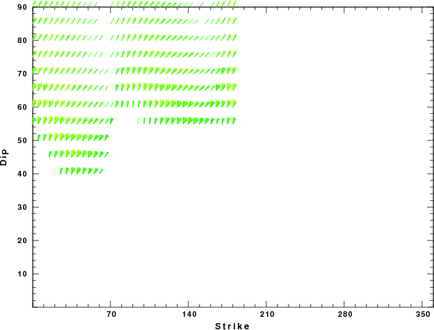
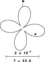
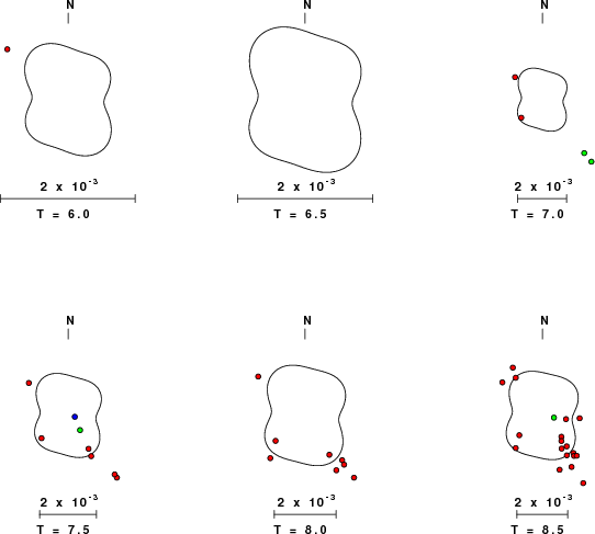
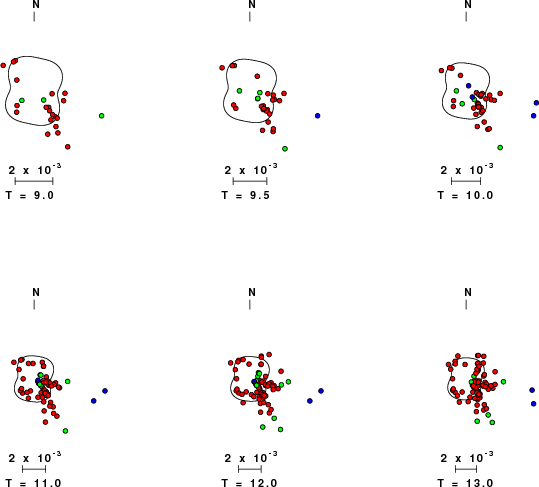
| Focal mechanism sensitivity at the preferred depth. The red color indicates a very good fit to thewavefroms. Each solution is plotted as a vector at a given value of strike and dip with the angle of the vector representing the rake angle, measured, with respect to the upward vertical (N) in the figure. |
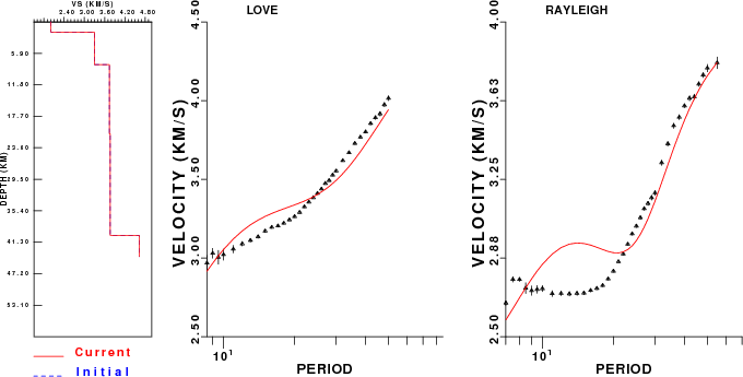
The following figure shows the stations used in the grid search for the best focal mechanism to fit the surface-wave spectral amplitudes of the Love and Rayleigh waves.
|
|
|
The surface-wave determined focal mechanism is shown here.
  NODAL PLANES


  STK=      91.87
  DIP=      68.53
 RAKE=     147.50

             OR

  STK=     194.99
  DIP=      60.00
 RAKE=      25.00


DEPTH = 19.0 km

Mw = 4.55
Best Fit 0.7447 - P-T axis plot gives solutions with FIT greater than FIT90
 |
The P-wave first motion data for focal mechanism studies are as follow:
Sta Az(deg)    Dist(km)   First motion
CWF       226   93 -12345
HPK       310  112 -12345
SWN1      207  225 -12345
MCH1      232  234 -12345
GAL1      303  335 -12345
EDI       328  344 -12345
HTL       229  385 -12345
DSB       271  405 -12345
DYA       219  406 -12345
JSA       197  478 -12345
WTSB      105  504 -12345
HGN       121  514 -12345
WLF       130  605 -12345
Surface wave analysis was performed using codes from Computer Programs in Seismology, specifically the multiple filter analysis program do_mft and the surface-wave radiation pattern search program srfgrd96.
Digital data were collected, instrument response removed and traces converted
to Z, R an T components. Multiple filter analysis was applied to the Z and T traces to obtain the Rayleigh- and Love-wave spectral amplitudes, respectively.
These were input to the search program which examined all depths between 1 and 25 km
and all possible mechanisms.
|
|
|

|
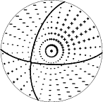
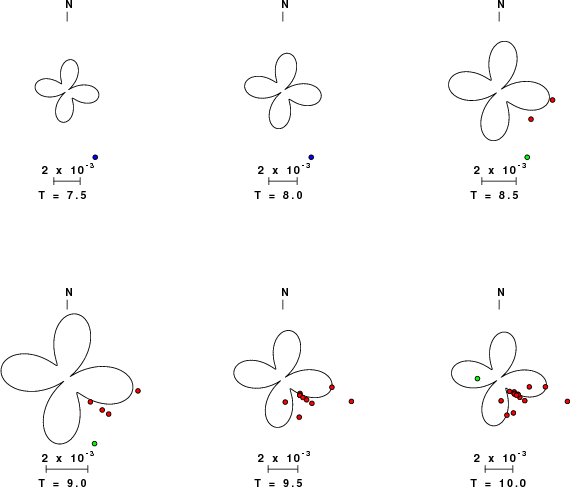
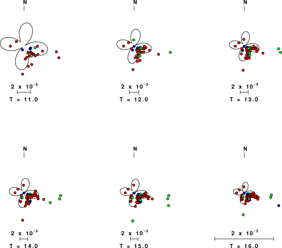
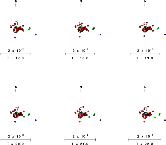
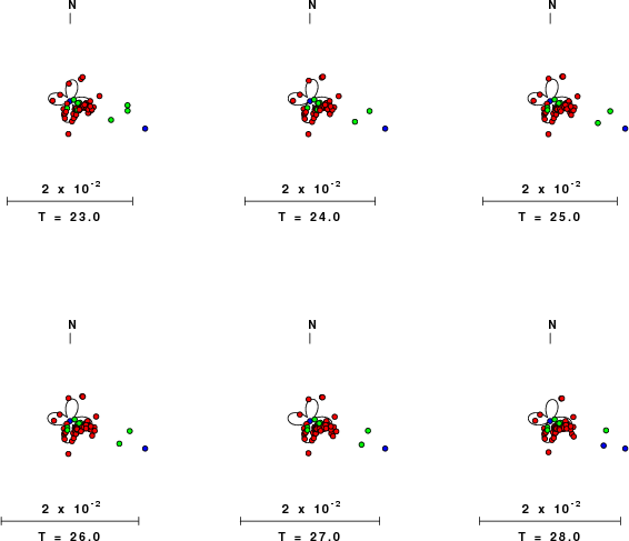
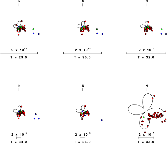
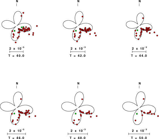
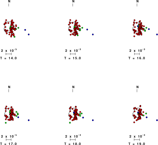
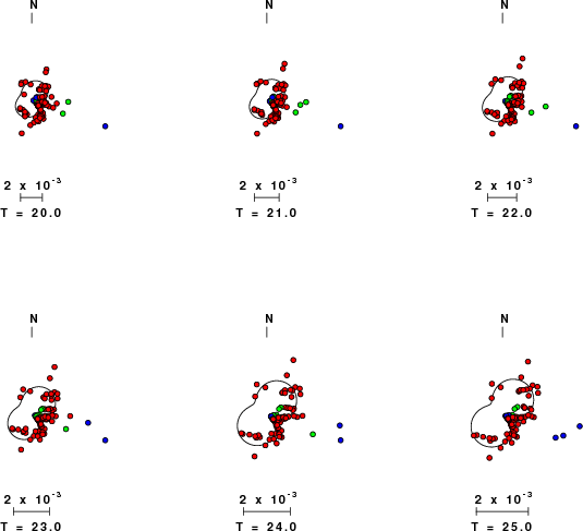
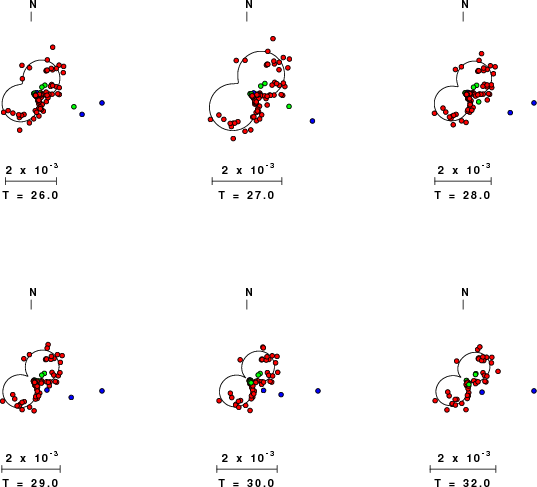
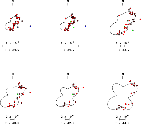
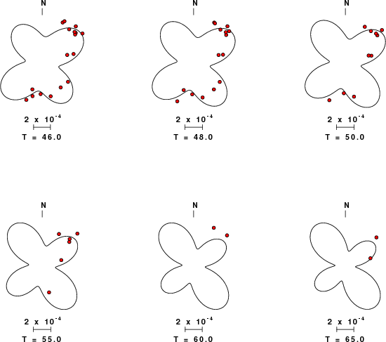
| Pressure-tension axis trends. Since the surface-wave spectra search does not distinguish between P and T axes and since there is a 180 ambiguity in strike, all possible P and T axes are plotted. First motion data and waveforms will be used to select the preferred mechanism. The purpose of this plot is to provide an idea of the possible range of solutions. The P and T-axes for all mechanisms with goodness of fit greater than 0.9 FITMAX (above) are plotted here. |
|
| Focal mechanism sensitivity at the preferred depth. The red color indicates a very good fit to the Love and Rayleigh wave radiation patterns. Each solution is plotted as a vector at a given value of strike and dip with the angle of the vector representing the rake angle, measured, with respect to the upward vertical (N) in the figure. Because of the symmetry of the spectral amplitude rediation patterns, only strikes from 0-180 degrees are sampled. |
The distribution of broadband stations with azimuth and distance is
Sta Az(deg)    Dist(km)
HPK	  310	  112
SWN1	  207	  225
MCH1	  232	  234
GAL1	  303	  335
EDI	  328	  344
HTL	  230	  385
NE05	  108	  395
DSB	  271	  405
DYA	  219	  406
OPLO	  112	  458
WIT	   94	  471
JSA	  196	  478
WTSB	  104	  504
HLG	   77	  549
IBBN	   98	  555
BUG	  109	  556
KPL	  325	  561
WLF	  130	  605
MUD	   56	  701
BSEG	   80	  706
LRW	  356	  761
ECH	  134	  774
BFO	  129	  823
STU	  123	  836
BOURR	  138	  849
BRANT	  143	  859
COP	   67	  865
MOX	  105	  870
BALST	  136	  875
CFF	  162	  876
SLE	  131	  877
SULZ	  134	  878
GIMEL	  145	  889
TORNY	  142	  894
RGN	   76	  904
ZUR	  133	  914
WILA	  131	  927
KONO	   37	  930
WIMIS	  139	  932
MANZ	  108	  934
AIGLE	  143	  935
NKC	  106	  944
SENIN	  142	  947
HASLI	  137	  948
BNALP	  136	  950
RUE	   90	  951
MUO	  134	  952
ROTZ	  110	  952
EMV	  144	  959
LIENZ	  130	  966
DIX	  142	  978
LLS	  134	  980
PLONS	  131	  981
DAVA	  129	  987
FUR	  120	  997
FUSIO	  136	  998
MMK	  140	 1004
BSD	   72	 1011
BRG	  100	 1012
DAVOX	  131	 1028
WET	  112	 1030
VDL	  134	 1032
BNI	  148	 1050
SOFL	  341	 1051
FETA	  127	 1053
FUORN	  130	 1061
MUGIO	  137	 1063
BERNI	  132	 1067
OGAG	  150	 1072
KHC	  110	 1074
RUSF	  156	 1126
OGDI	  152	 1130
GKP	   83	 1167
KSP	   97	 1168
ARBF	  157	 1169
ABTA	  124	 1171
CALF	  151	 1189
KBA	  120	 1194
MOA	  115	 1195
ESCA	  149	 1196
ANTF	  150	 1215
CSOR	  174	 1222
EJON	  168	 1232
MYKA	  121	 1244
KRUC	  105	 1256
VRAC	  104	 1256
VLC	  138	 1284
CONA	  111	 1288
CSNA	  111	 1288
MORC	  100	 1296
OBKA	  120	 1305
ARSA	  115	 1311
SOKA	  118	 1321
OKC	  100	 1332
SOP	  111	 1346
JAVC	  104	 1349
ECAL	  203	 1353
OJC	   96	 1425
VYHS	  104	 1444
BUD	  108	 1514
MAHO	  165	 1532
MTE	  204	 1537
SUW	   78	 1547
PKSM	  113	 1571
RAF	   48	 1575
CRVS	   99	 1595
MEF	   53	 1681
PESTR	  202	 1700
VAF	   42	 1716
EMUR	  183	 1722
VSU	   60	 1772
DRGR	  105	 1791
DIVS	  116	 1802
PVAQ	  201	 1859
SUF	   45	 1861
SFS	  196	 1928
OUL	   38	 1964
TIR	  104	 2011
HEF	   28	 2096
VTS	  115	 2107
JOF	   47	 2117
RTC	  196	 2210
ARE0	   26	 2236
TIRR	  104	 2305
RDO	  115	 2358
OBN	   70	 2386
IDI	  125	 2810
LAST	  125	 2853
ISP	  114	 2920
CSS	  114	 3327
Since the analysis of the surface-wave radiation patterns uses only spectral amplitudes and because the surfave-wave radiation patterns have a 180 degree symmetry, each surface-wave solution consists of four possible focal mechanisms corresponding to the interchange of the P- and T-axes and a roation of the mechanism by 180 degrees. To select one mechanism, P-wave first motion can be used. This was not possible in this case because all the P-wave first motions were emergent ( a feature of the P-wave wave takeoff angle, the station location and the mechanism). The other way to select among the mechanisms is to compute forward synthetics and compare the observed and predicted waveforms.
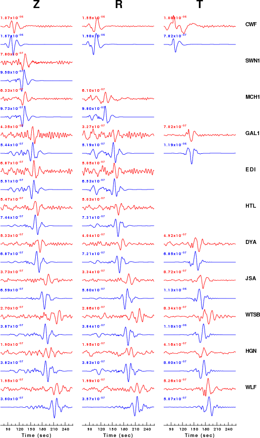
The fits to the waveforms with the given mechanism are show below:
|
This figure shows the fit to the three components of motion (Z - vertical, R-radial and T - transverse). For each station and component, the observed traces is shown in red and the model predicted trace in blue. The traces represent filtered ground velocity in units of meters/sec (the peak value is printed adjacent to each trace; each pair of traces to plotted to the same scale to emphasize the difference in levels). Both synthetic and observed traces have been filtered using the SAC commands:
hp c 0.02 n 3
lp c 0.05 n 3
|

|
Should the national backbone of the USGS Advanced National Seismic System (ANSS) be implemented with an interstation separation of 300 km, it is very likely that an earthquake such as this would have been recorded at distances on the order of 100-200 km. This means that the closest station would have information on source depth and mechanism that was lacking here.
Dr. Harley Benz, USGS, provided the USGS USNSN digital data. The digital data used in this study were provided by Natural Resources Canada through their AUTODRM site http://www.seismo.nrcan.gc.ca/nwfa/autodrm/autodrm_req_e.php, and IRIS using their BUD interface.
Thanks also to the many seismic network operators whose dedication make this effort possible: University of Alaska, University of Washington, Oregon State University, University of Utah, Montana Bureas of Mines, UC Berkely, Caltech, UC San Diego, Saint L ouis University, Universityof Memphis, Lamont Doehrty Earth Observatory, Boston College, the Iris stations and the Transportable Array of EarthScope.
The VELOCITY_MODEL used for the waveform synthetic seismograms and for the surface wave eigenfunctions and dispersion is as follows:
Here we tabulate the reasons for not using certain digital data sets
The following stations did not have a valid response files:
DATE=Wed Feb 27 15:54:00 CST 2008