2007/04/28 07:18:11 51.02N 1.03W 10 4.7 England
USGS Felt map for this earthquake
USGS Felt reports page for Europe
SLU Moment Tensor Solution
2007/04/28 07:18:11 51.02N 1.03W 10 4.7 England
Best Fitting Double Couple
Mo = 7.76e+21 dyne-cm
Mw = 3.86
Z = 8 km
Plane Strike Dip Rake
NP1 80 70 70
NP2 307 28 133
Principal Axes:
Axis Value Plunge Azimuth
T 7.76e+21 60 321
N 0.00e+00 19 87
P -7.76e+21 22 185
Moment Tensor: (dyne-cm)
Component Value
Mxx -5.40e+21
Mxy -1.54e+21
Mxz 5.35e+21
Myy 7.12e+20
Myz -1.86e+21
Mzz 4.69e+21
--------------
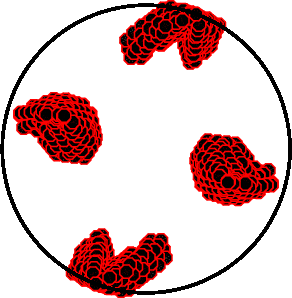
----------------------
----############------------
#####################---------
##########################--------
#############################-------
############ #################------
############# T ##################------
############# ####################----
#####################################----#
##########################################
###################################----###
###############################--------###
--#####################---------------##
--------------------------------------##
-------------------------------------#
-----------------------------------#
----------------------------------
------------ ---------------
----------- P --------------
-------- -----------
--------------
Harvard Convention
Moment Tensor:
R T F
4.69e+21 5.35e+21 1.86e+21
5.35e+21 -5.40e+21 1.54e+21
1.86e+21 1.54e+21 7.12e+20
Details of the solution is found at
http://www.eas.slu.edu/Earthquake_Center/MECH.NA/20070428071811/index.html
|
      STK = 80
      DIP = 70
     RAKE = 70
       MW = 3.86
       HS = 8
The waveform is preferred. The surface wave indiciates a similar size and ahsllow depth, but aximuth control is not great and some stations should not have been used, e.g., Spain because of Atlantic Ocean path.
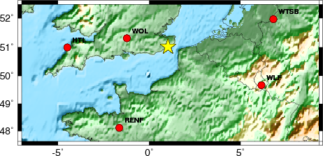
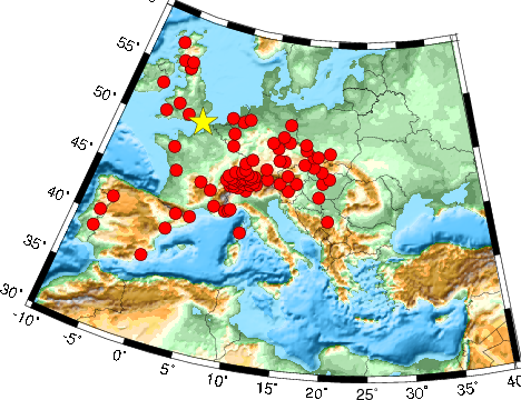
The focal mechanism was determined using broadband seismic waveforms. The location of the event and the and stations used for the waveform inversion are shown in the next figure.
|
|
|
|
The program wvfgrd96 was used with good traces observed at short distance to determine the focal mechanism, depth and seismic moment. This technique requires a high quality signal and well determined velocity model for the Green functions. To the extent that these are the quality data, this type of mechanism should be preferred over the radiation pattern technique which requires the separate step of defining the pressure and tension quadrants and the correct strike.
The observed and predicted traces are filtered using the following gsac commands:
hp c 0.02 n 3
lp c 0.05 n 3
The results of this grid search from 0.5 to 19 km depth are as follow:
           DEPTH  STK   DIP  RAKE   MW    FIT
WVFGRD96    0.5    65    80    65   3.75 0.2448
WVFGRD96    1.0    65    75    55   3.67 0.2565
WVFGRD96    2.0   320    75   -60   3.78 0.2989
WVFGRD96    3.0    70    75    60   3.80 0.3465
WVFGRD96    4.0    75    70    60   3.81 0.3627
WVFGRD96    5.0    75    70    60   3.81 0.3732
WVFGRD96    6.0    75    70    60   3.81 0.3748
WVFGRD96    7.0    80    70    65   3.82 0.3737
WVFGRD96    8.0    80    70    70   3.86 0.3791
WVFGRD96    9.0    85    70    75   3.88 0.3771
WVFGRD96   10.0    85    70    75   3.88 0.3762
WVFGRD96   11.0    85    70    80   3.88 0.3744
WVFGRD96   12.0    85    70    80   3.87 0.3723
WVFGRD96   13.0   155    20   -20   3.85 0.3719
WVFGRD96   14.0   160    20   -15   3.85 0.3725
WVFGRD96   15.0   160    20   -15   3.85 0.3733
WVFGRD96   16.0   165    20   -10   3.85 0.3740
WVFGRD96   17.0   165    20   -10   3.85 0.3741
WVFGRD96   18.0   170    20    -5   3.85 0.3744
WVFGRD96   19.0   170    20    -5   3.85 0.3741
WVFGRD96   20.0   180    15     5   3.85 0.3742
WVFGRD96   21.0    85    80    85   3.92 0.3755
WVFGRD96   22.0    85    85    95   3.92 0.3723
WVFGRD96   23.0    85    85    90   3.93 0.3694
WVFGRD96   24.0   265     5    90   3.93 0.3662
WVFGRD96   25.0   265     5    90   3.94 0.3631
WVFGRD96   26.0    85    85    85   3.94 0.3595
WVFGRD96   27.0    85    85    85   3.94 0.3560
WVFGRD96   28.0    85    85    85   3.95 0.3530
WVFGRD96   29.0    85    85    80   3.95 0.3482
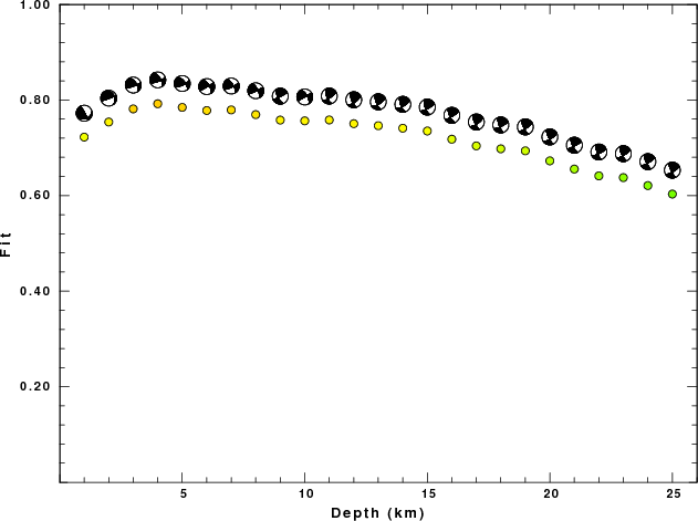
The best solution is
WVFGRD96 8.0 80 70 70 3.86 0.3791
The mechanism correspond to the best fit is
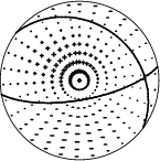
|
|
|
The best fit as a function of depth is given in the following figure:
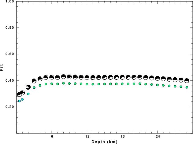
|
|
|
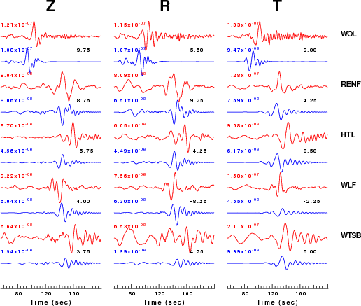
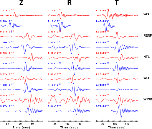
The comparison of the observed and predicted waveforms is given in the next figure. The red traces are the observed and the blue are the predicted. Each observed-predicted componnet is plotted to the same scale and peak amplitudes are indicated by the numbers to the left of each trace. The number in black at the rightr of each predicted traces it the time shift required for maximum correlation between the observed and predicted traces. This time shift is required because the synthetics are not computed at exactly the same distance as the observed and because the velocity model used in the predictions may not be perfect. A positive time shift indicates that the prediction is too fast and should be delayed to match the observed trace (shift to the right in this figure). A negative value indicates that the prediction is too slow. The bandpass filter used in the processing and for the display was
hp c 0.02 n 3
lp c 0.05 n 3
|
|
|
|
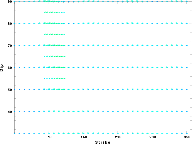
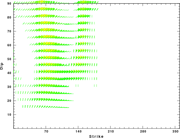
| Focal mechanism sensitivity at the preferred depth. The red color indicates a very good fit to thewavefroms. Each solution is plotted as a vector at a given value of strike and dip with the angle of the vector representing the rake angle, measured, with respect to the upward vertical (N) in the figure. |
The following figure shows the stations used in the grid search for the best focal mechanism to fit the surface-wave spectral amplitudes of the Love and Rayleigh waves.
|
|
|
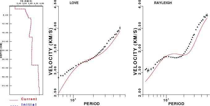
The surface-wave determined focal mechanism is shown here.
  NODAL PLANES


  STK=      69.99
  DIP=      70.00
 RAKE=      34.99

             OR

  STK=     326.52
  DIP=      57.39
 RAKE=     156.04


DEPTH = 4.0 km

Mw = 3.96
Best Fit 0.7622 - P-T axis plot gives solutions with FIT greater than FIT90
 |
The P-wave first motion data for focal mechanism studies are as follow:
Sta Az(deg)    Dist(km)   First motion
WOL       282  161 -12345
SWN       287  205 -12345
DOU       111  273 -12345
MCH       293  300 -12345
RENF      212  376 -12345
HTL       272  387 -12345
WLF       110  394 -12345
WTSB       73  414 -12345
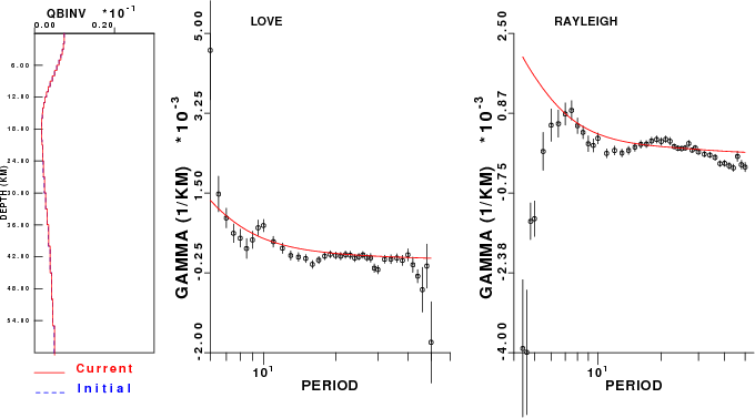
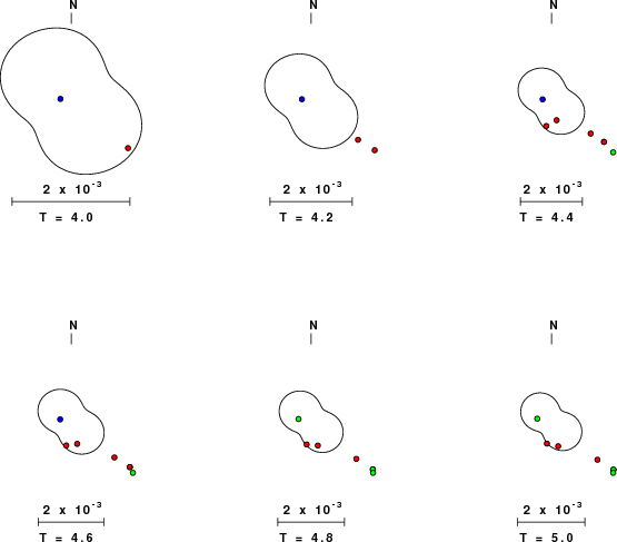
Surface wave analysis was performed using codes from Computer Programs in Seismology, specifically the multiple filter analysis program do_mft and the surface-wave radiation pattern search program srfgrd96.
The velocity model used for the search is a modified Utah model .
Digital data were collected, instrument response removed and traces converted
to Z, R an T components. Multiple filter analysis was applied to the Z and T traces to obtain the Rayleigh- and Love-wave spectral amplitudes, respectively.
These were input to the search program which examined all depths between 1 and 25 km
and all possible mechanisms.
|
|
|
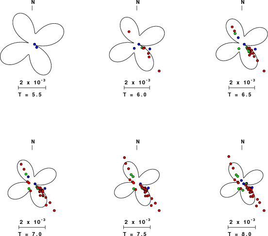
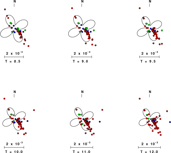
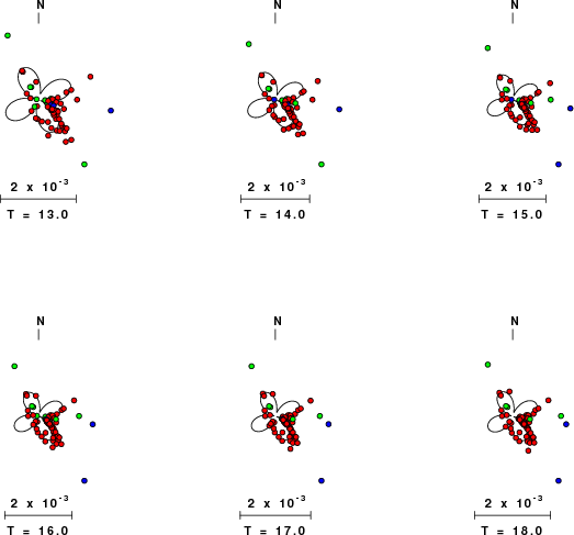
|
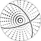
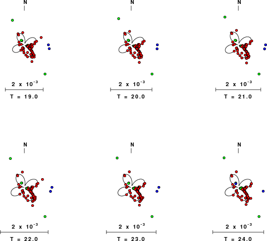
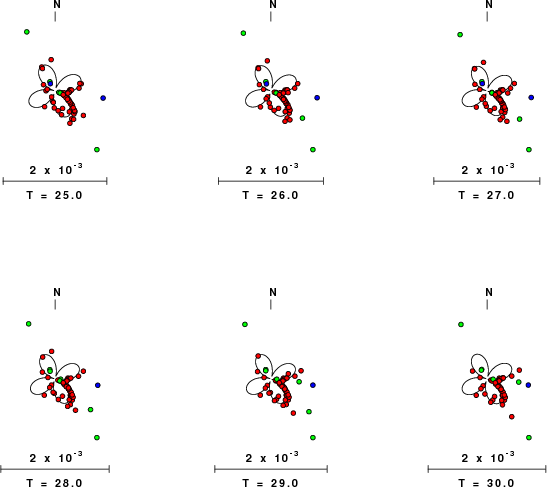
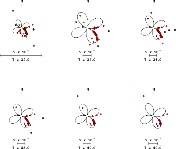
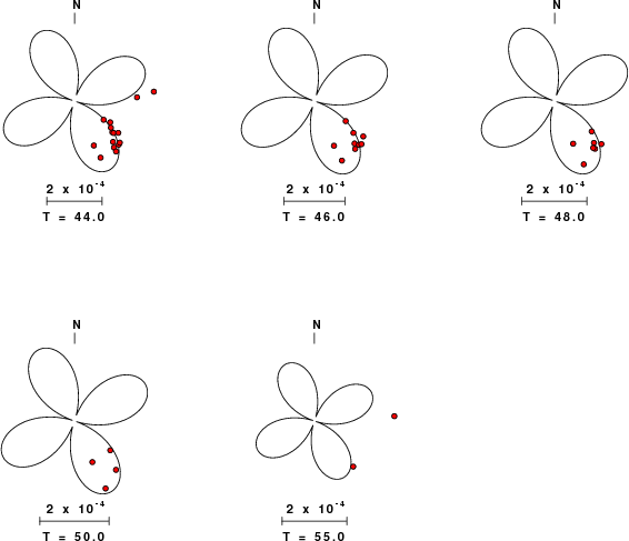
| Pressure-tension axis trends. Since the surface-wave spectra search does not distinguish between P and T axes and since there is a 180 ambiguity in strike, all possible P and T axes are plotted. First motion data and waveforms will be used to select the preferred mechanism. The purpose of this plot is to provide an idea of the possible range of solutions. The P and T-axes for all mechanisms with goodness of fit greater than 0.9 FITMAX (above) are plotted here. |
|
| Focal mechanism sensitivity at the preferred depth. The red color indicates a very good fit to the Love and Rayleigh wave radiation patterns. Each solution is plotted as a vector at a given value of strike and dip with the angle of the vector representing the rake angle, measured, with respect to the upward vertical (N) in the figure. Because of the symmetry of the spectral amplitude rediation patterns, only strikes from 0-180 degrees are sampled. |
Sta Az(deg)    Dist(km)
WOL	  282	  161
MCH	  293	  300
NE05	   66	  311
HGN	   93	  346
RENF	  212	  376
HTL	  272	  387
WLF	  110	  394
WTSB	   73	  414
IBBN	   70	  487
CHIF	  192	  554
ESK	  331	  556
EKB	  331	  557
DSB	  299	  564
BRANT	  137	  604
CFF	  164	  604
BFO	  117	  605
BOURR	  129	  605
EDI	  334	  613
GIMEL	  140	  630
BALST	  128	  635
STU	  110	  637
TORNY	  135	  641
SULZ	  124	  645
PGB	  328	  646
SLE	  121	  651
AIGLE	  138	  678
ZUR	  124	  683
WIMIS	  132	  684
SSB	  156	  690
SENIN	  136	  693
WILA	  122	  699
EMV	  140	  701
HASLI	  130	  705
BNALP	  128	  711
MUO	  126	  716
DIX	  137	  723
LIENZ	  121	  743
LLS	  125	  746
MOX	   89	  746
MMK	  134	  753
PLONS	  123	  753
FUSIO	  129	  756
DAVA	  119	  767
VDL	  126	  798
DAVOX	  123	  801
FUR	  109	  805
NKC	   92	  812
MUGIO	  131	  819
KPL	  331	  827
FUORN	  122	  835
CLL	   83	  837
RUSF	  155	  855
WET	   99	  872
WTTA	  114	  878
RUE	   75	  894
BRG	   86	  907
KHC	   98	  921
CALF	  149	  922
SAOF	  145	  923
ESCA	  147	  931
CSOR	  180	  961
EJON	  171	  963
KBA	  111	 1000
MOA	  105	 1021
LRW	  353	 1024
KSP	   85	 1071
DPC	   88	 1087
OBKA	  112	 1111
KRUC	   95	 1120
EBR	  182	 1134
ARSA	  106	 1135
ECAL	  214	 1171
SMPL	  144	 1175
MORC	   90	 1180
JAVC	   95	 1216
OKC	   90	 1221
VYHS	   96	 1310
OJC	   86	 1328
MTE	  213	 1354
BUD	  100	 1364
PKSM	  106	 1400
PSZ	   97	 1406
EMUR	  188	 1475
PESTR	  210	 1510
DIVS	  111	 1615
RAF	   41	 1693
MEF	   46	 1778
ARE0	   23	 2430
Since the analysis of the surface-wave radiation patterns uses only spectral amplitudes and because the surfave-wave radiation patterns have a 180 degree symmetry, each surface-wave solution consists of four possible focal mechanisms corresponding to the interchange of the P- and T-axes and a roation of the mechanism by 180 degrees. To select one mechanism, P-wave first motion can be used. This was not possible in this case because all the P-wave first motions were emergent ( a feature of the P-wave wave takeoff angle, the station location and the mechanism). The other way to select among the mechanisms is to compute forward synthetics and compare the observed and predicted waveforms.
The velocity model used for the waveform fit is a modified Utah model .
The fits to the waveforms with the given mechanism are show below:
|
This figure shows the fit to the three components of motion (Z - vertical, R-radial and T - transverse). For each station and component, the observed traces is shown in red and the model predicted trace in blue. The traces represent filtered ground velocity in units of meters/sec (the peak value is printed adjacent to each trace; each pair of traces to plotted to the same scale to emphasize the difference in levels). Both synthetic and observed traces have been filtered using the SAC commands:
hp c 0.02 n 3
lp c 0.05 n 3
|
|
Should the national backbone of the USGS Advanced National Seismic System (ANSS) be implemented with an interstation separation of 300 km, it is very likely that an earthquake such as this would have been recorded at distances on the order of 100-200 km. This means that the closest station would have information on source depth and mechanism that was lacking here.
Dr. Harley Benz, USGS, provided the USGS USNSN digital data. The digital data used in this study were provided by Natural Resources Canada through their AUTODRM site http://www.seismo.nrcan.gc.ca/nwfa/autodrm/autodrm_req_e.php, and IRIS using their BUD interface
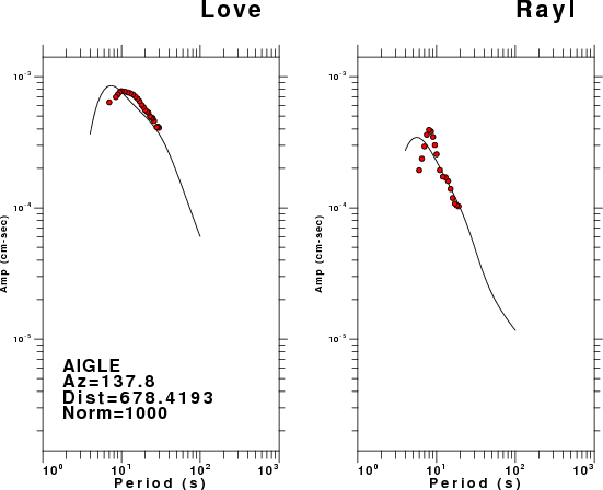
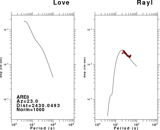
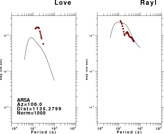
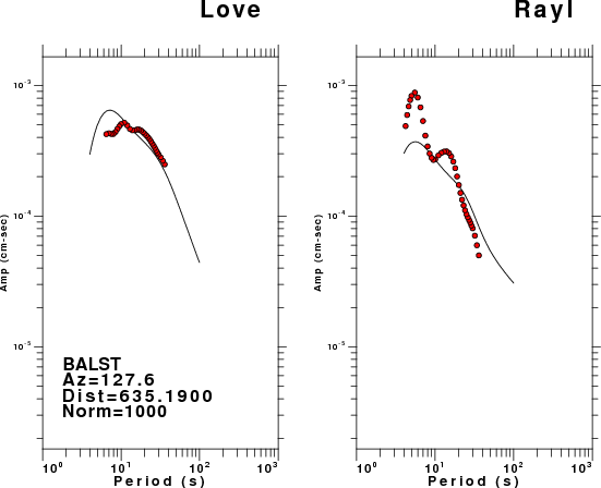
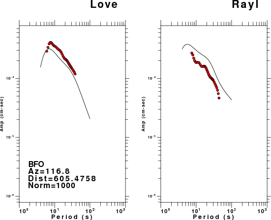
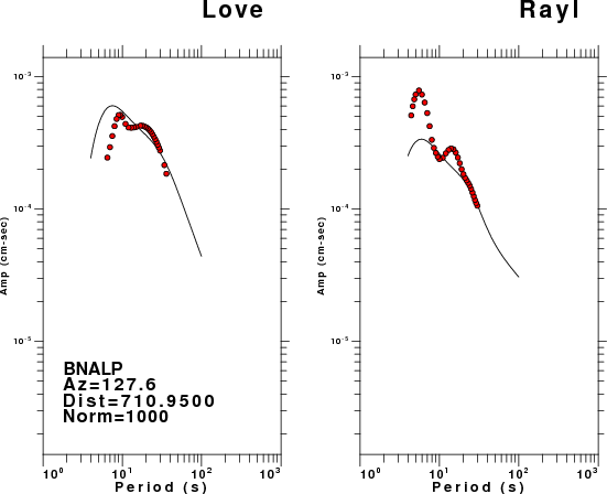
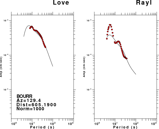
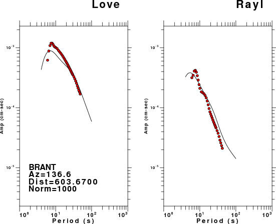
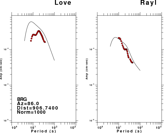
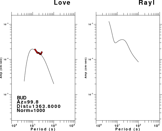
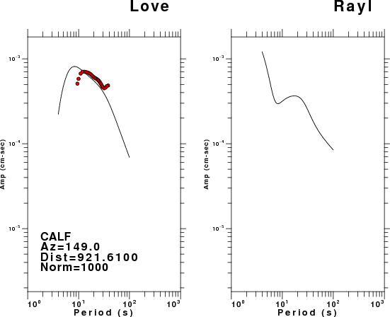
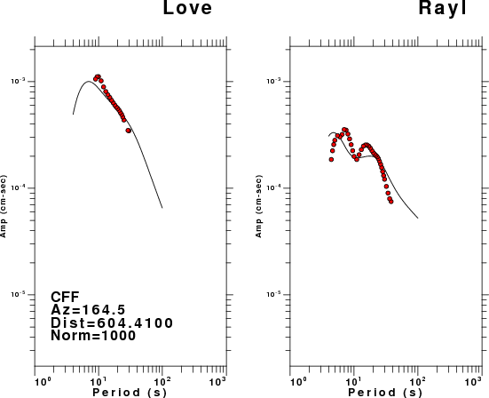
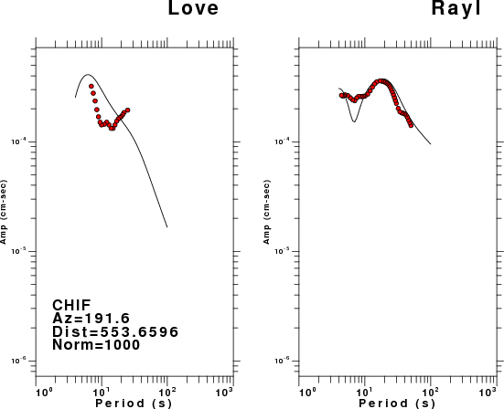
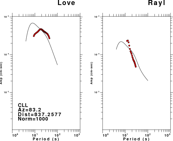
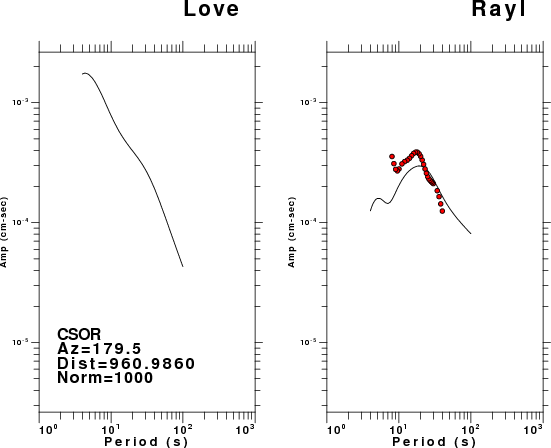
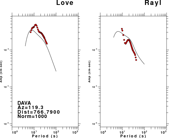
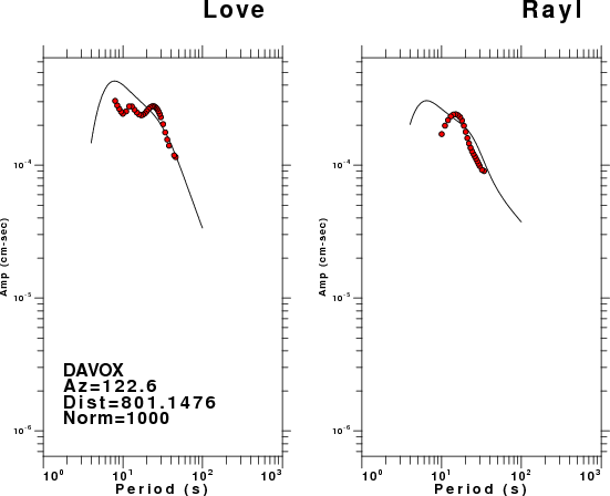
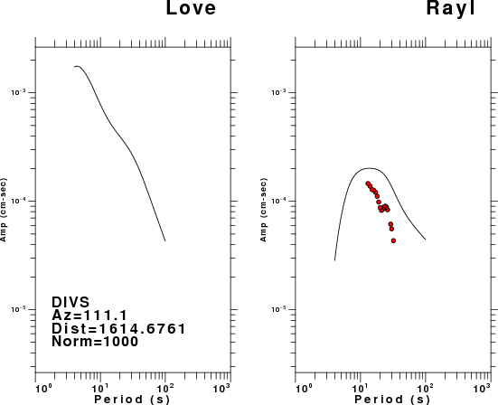
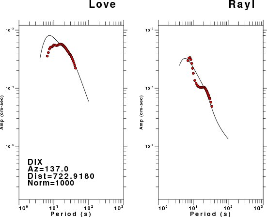
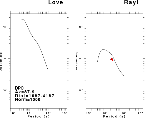
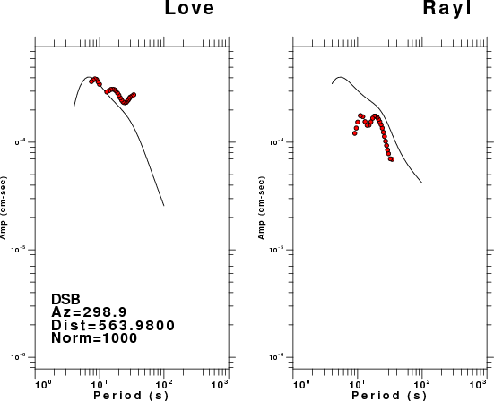
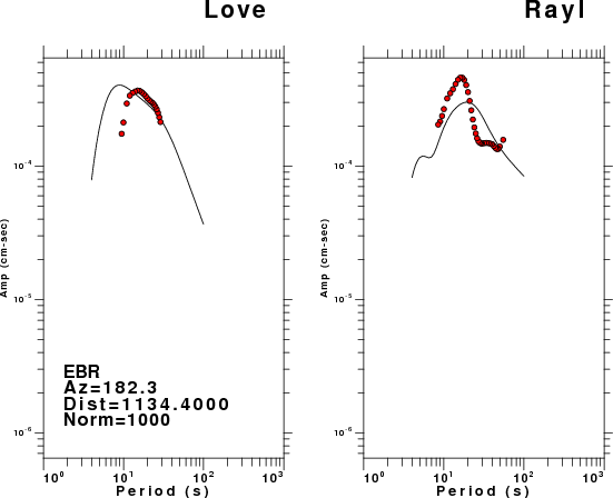
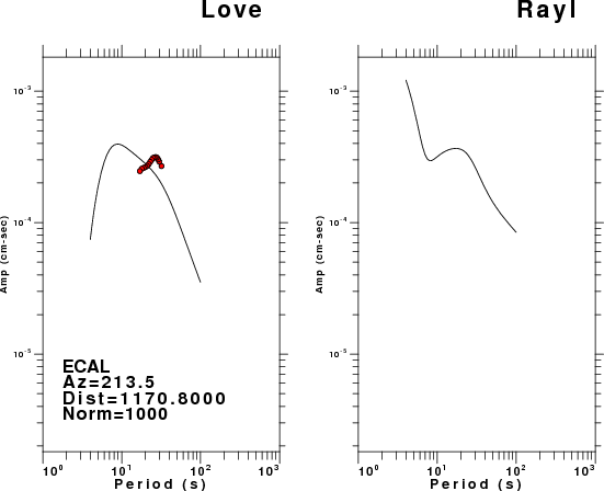
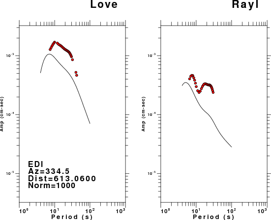
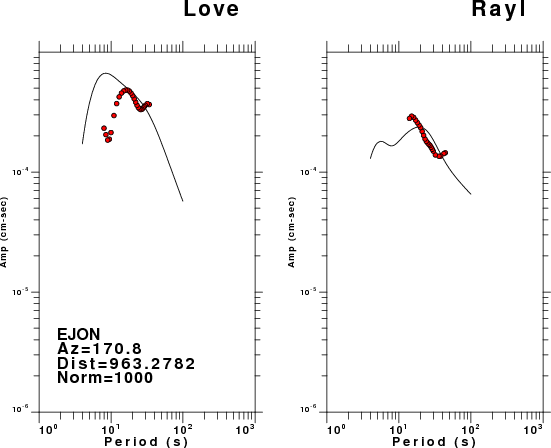
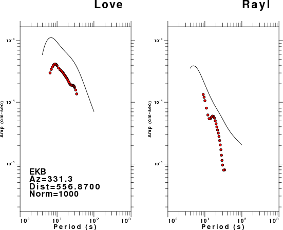
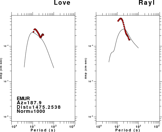
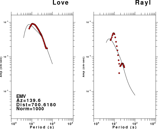
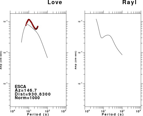
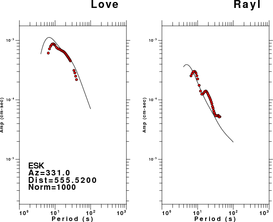
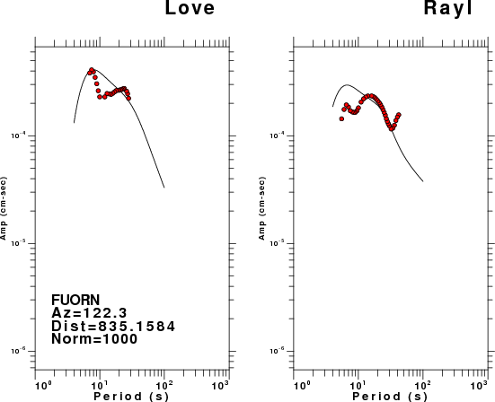
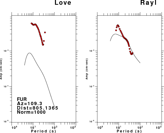
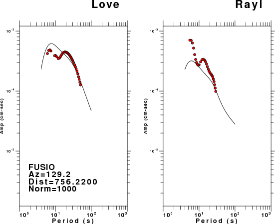
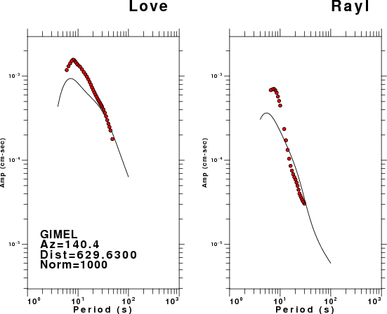
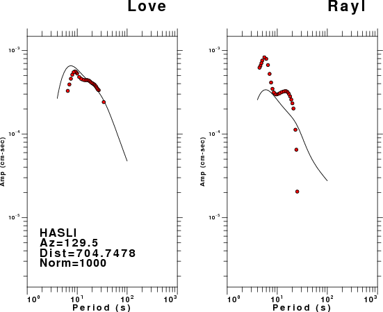
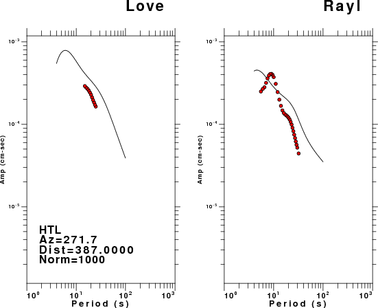
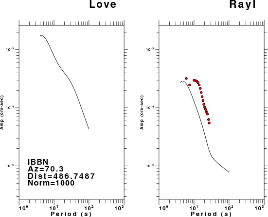
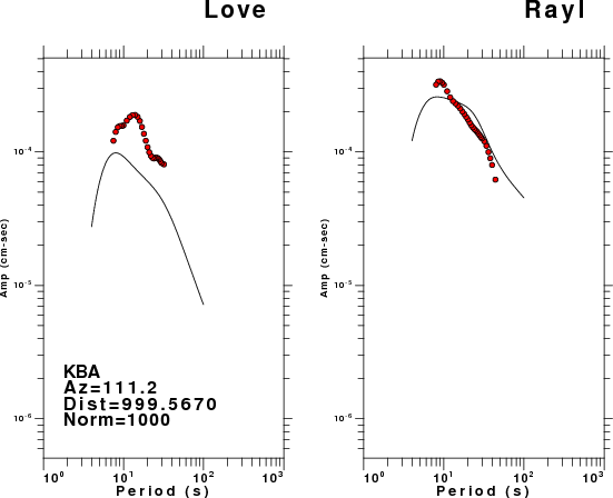
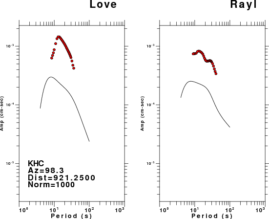
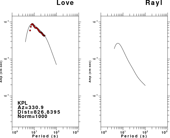
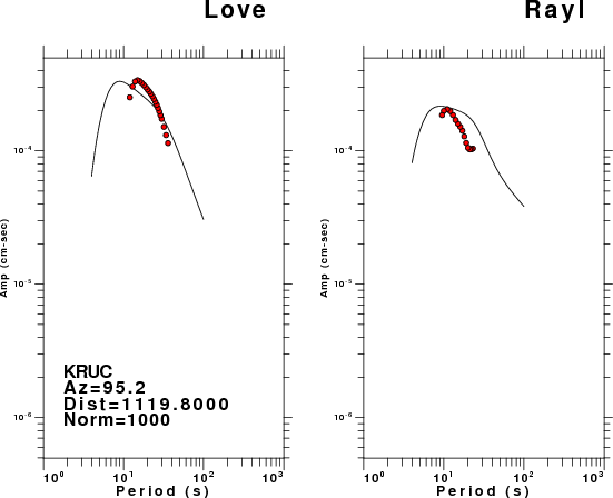
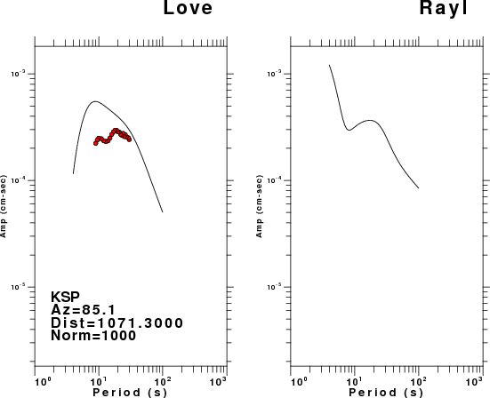
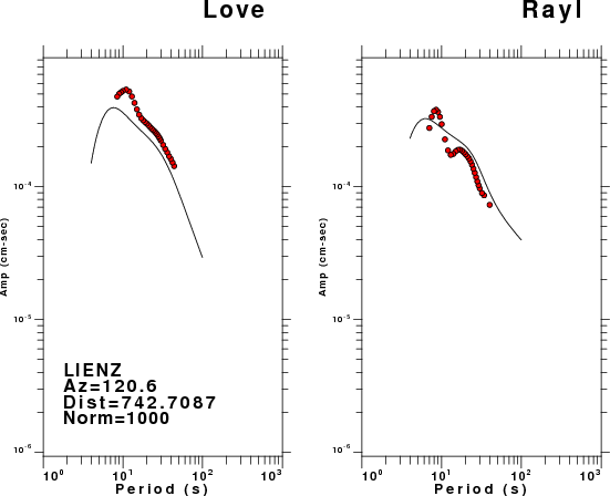
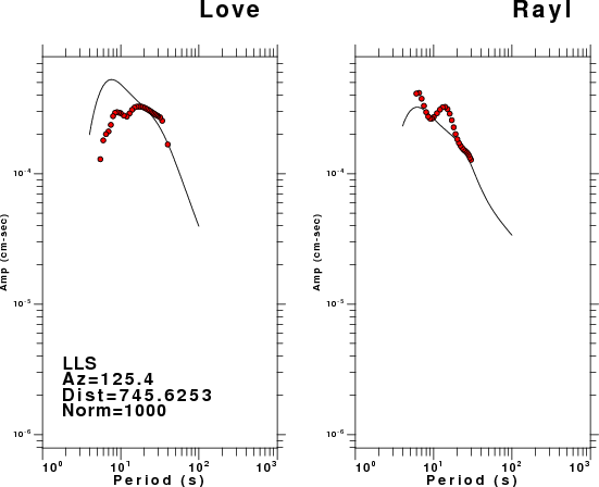
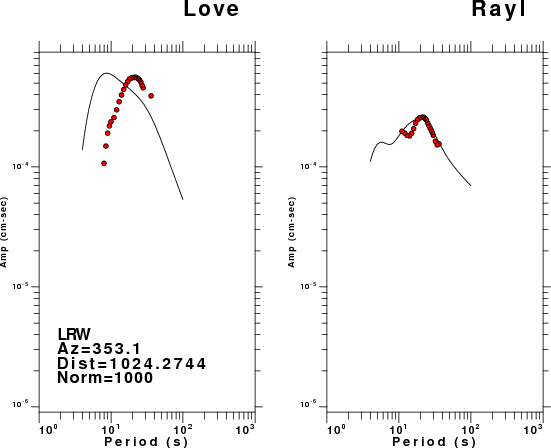
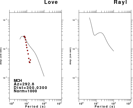
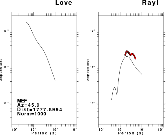
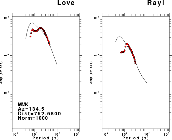
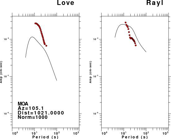
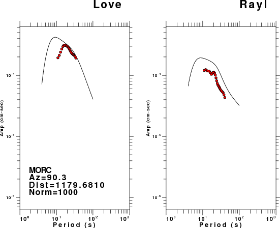
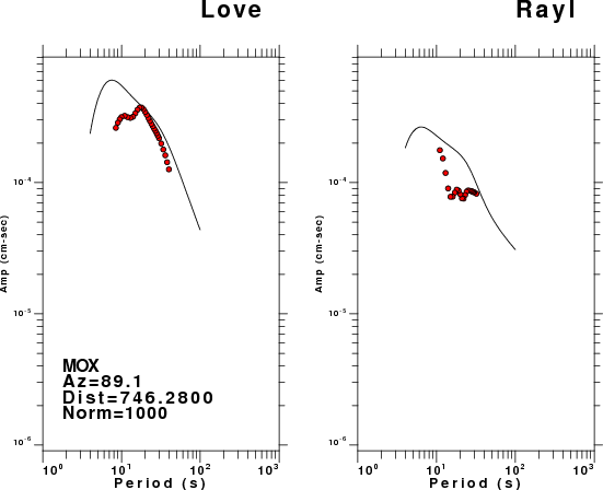
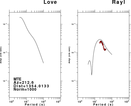
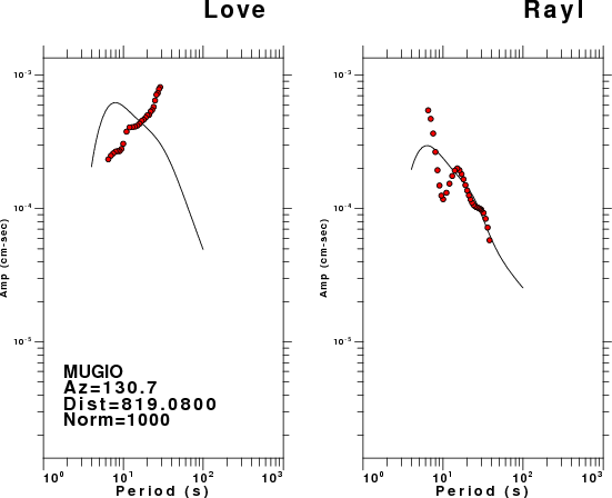
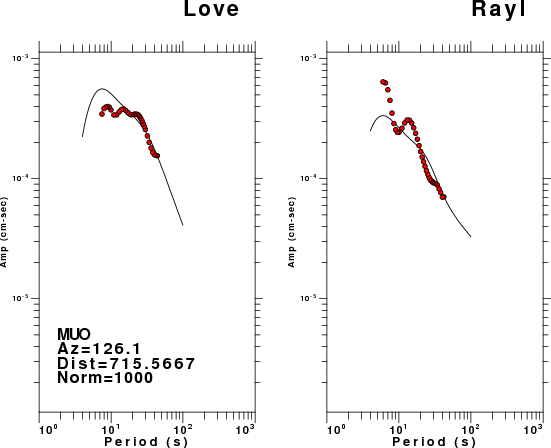
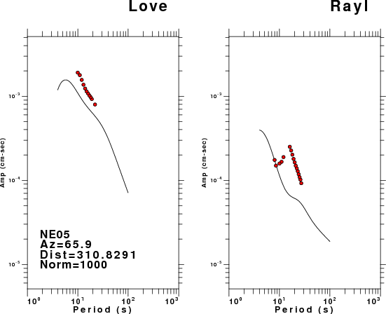
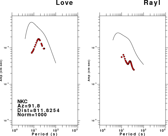
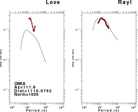
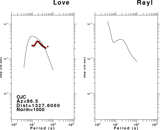
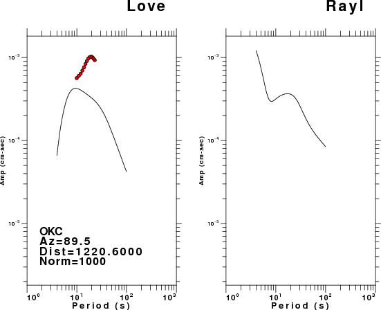
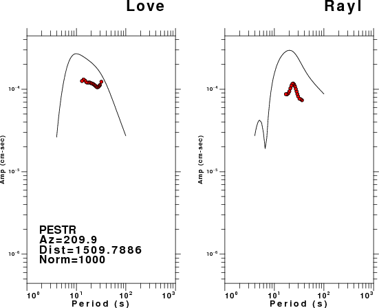
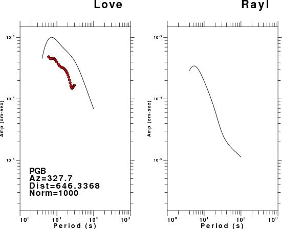
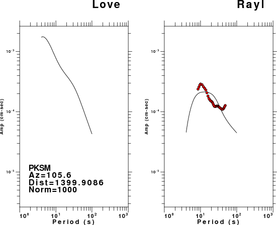
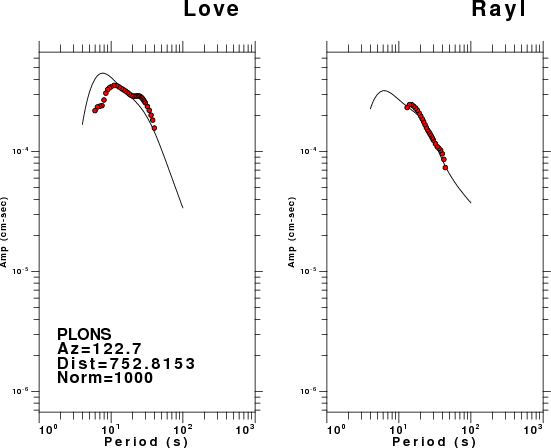
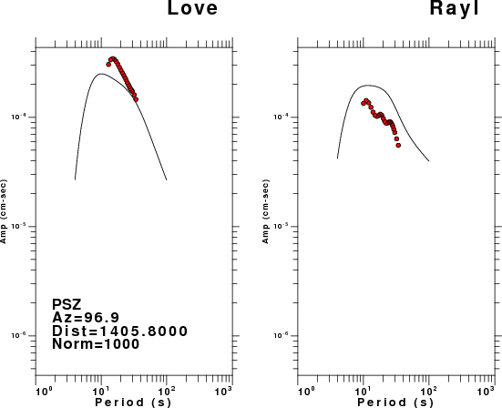
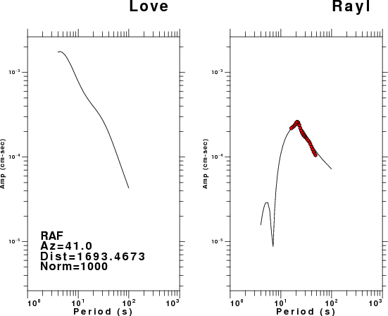
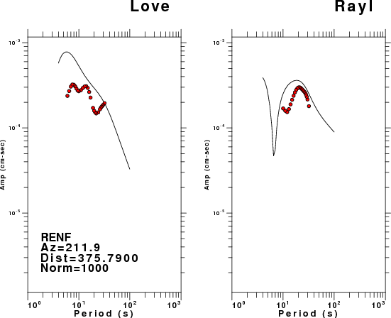
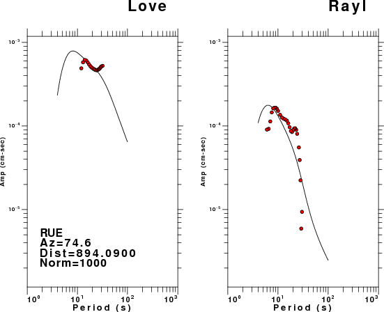
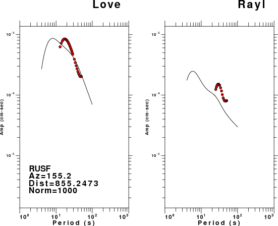
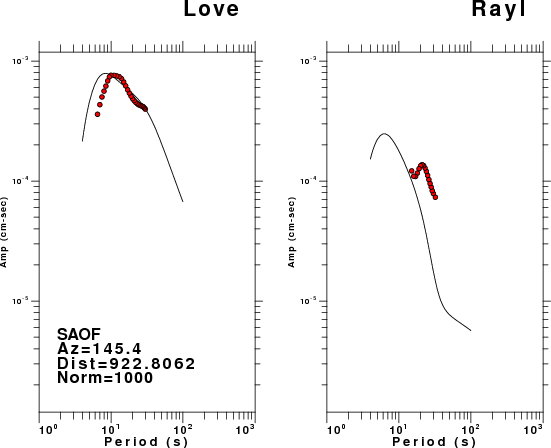
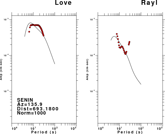
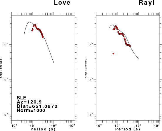
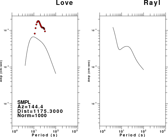
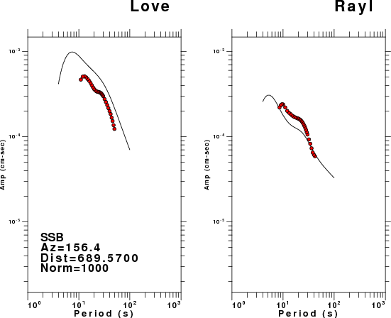
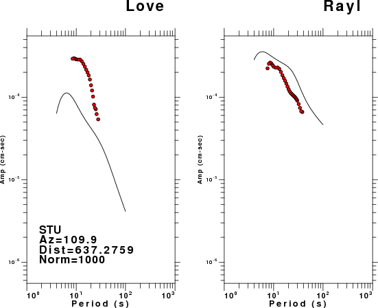
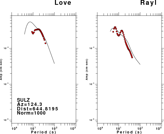
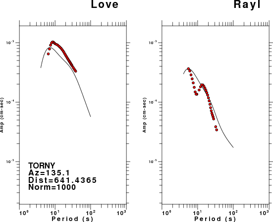
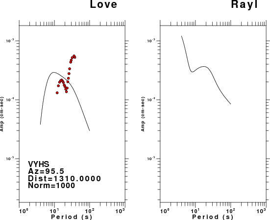
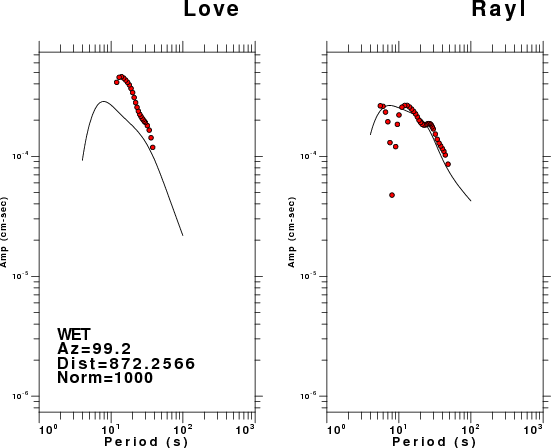
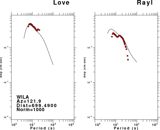
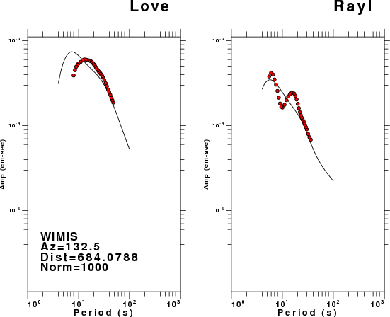
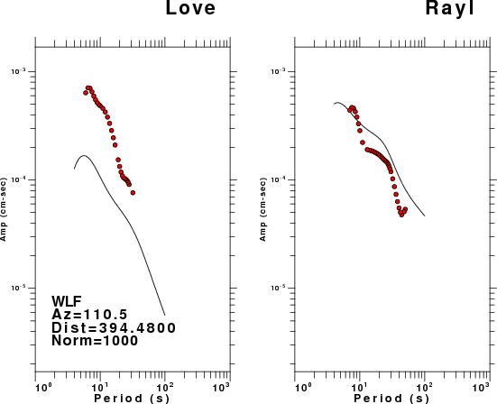
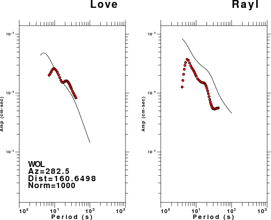
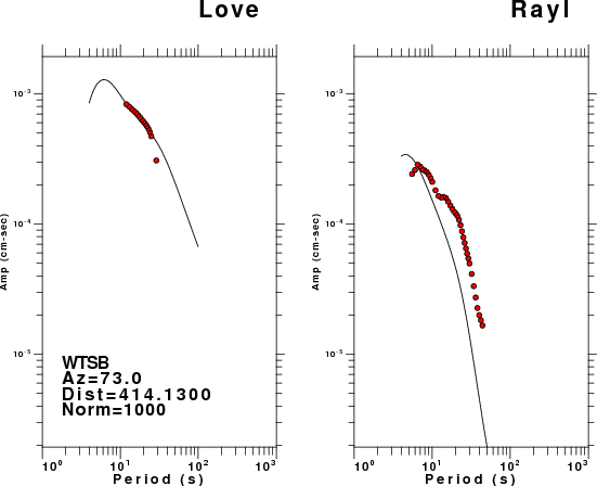
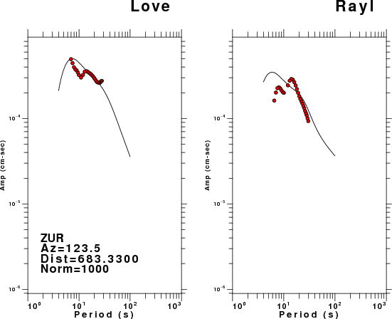
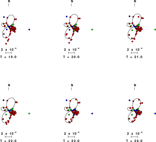
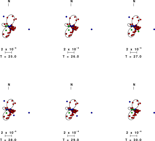
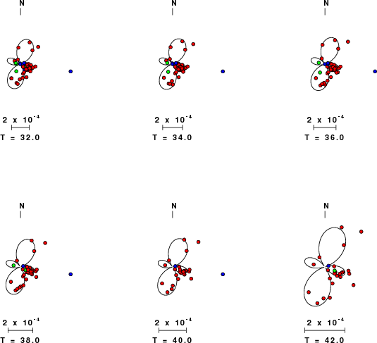
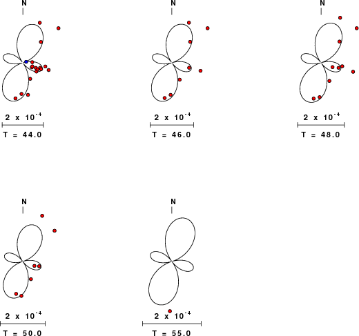
The figures below show the observed spectral amplitudes (units of cm-sec) at each station and the
theoretical predictions as a function of period for the mechanism given above. The modified Utah model earth model
was used to define the Green's functions. For each station, the Love and Rayleigh wave spectrail amplitudes are plotted with the same scaling so that one can get a sense fo the effects of the effects of the focal mechanism and depth on the excitation of each.
 |
 |
 |
 |
 |
 |
 |
 |
 |
 |
 |
 |
 |
 |
 |
 |
 |
 |
 |
 |
 |
 |
 |
 |
 |
 |
 |
 |
 |
 |
 |
 |
 |
 |
 |
 |
 |
 |
 |
 |
 |
 |
 |
 |
 |
 |
 |
 |
 |
 |
 |
 |
 |
 |
 |
 |
 |
 |
 |
 |
 |
 |
 |
 |
 |
 |
 |
 |
 |
 |
 |
 |
 |
 |
 |
 |
 |
 |
 |
 |
 |
 |
 |
 |
 |
 |
 |
 |
Here we tabulate the reasons for not using certain digital data sets
The following stations did not have a valid response files: