2006/06/29 21:02:09 55.84N 26.97E 10 5.7 Iran
USGS Felt map for this earthquake
USGS Felt reports page for Iran
 SLU Moment Tensor Solution
 2006/06/29 21:02:09 55.84N 26.97E 10 5.7 Iran

 Best Fitting Double Couple
    Mo = 4.03e+24 dyne-cm
    Mw = 5.67
    Z  = 9 km
     Plane   Strike  Dip  Rake
      NP1       30    70    45
      NP2      281    48   153
 Principal Axes:
   Axis    Value   Plunge  Azimuth
     T   4.03e+24     45     255
     N   0.00e+00     42      49
     P  -4.03e+24     13     151


 Moment Tensor: (dyne-cm)
    Component  Value
       Mxx    -2.78e+24
       Mxy     2.13e+24
       Mxz     2.47e+23
       Myy     9.45e+23
       Myz    -2.38e+24
       Mzz     1.83e+24


                     --------------
                 ---------------------#
              ------------------------####
             -------------------------#####
           ---------------------------#######
          --------############--------########
         ----#######################-##########
        --###########################---########
        ############################------######
       ############################---------#####
       ###########################------------###
       #########   ##############--------------##
       ######### T #############----------------#
        ########   ############-----------------
        ######################------------------
         ####################------------------
          #################-------------------
           ##############--------------------
             ###########-----------   -----
              #######-------------- P ----
                 #-----------------   -
                     --------------


 Harvard Convention
 Moment Tensor:
      R          T          F
  1.83e+24   2.47e+23   2.38e+24
  2.47e+23  -2.78e+24  -2.13e+24
  2.38e+24  -2.13e+24   9.45e+23


Details of the solution is found at

http://www.eas.slu.edu/Earthquake_Center/MECH.EU/20060628210209/index.html
|
      STK = 30
      DIP = 70
     RAKE = 45
       MW = 5.67
       HS = 9.0
This is only the surface wave fit. Other solutions are at
http://www.eas.slu.edu/Earthquake_Center/MECH.TEL/20060628210209.all/HTML and
http://www.eas.slu.edu/Earthquake_Center/MECH.TEL/20060628210209/HTML
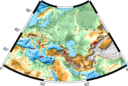
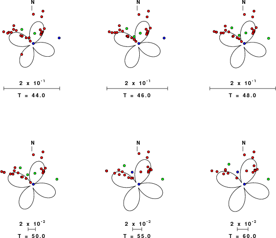
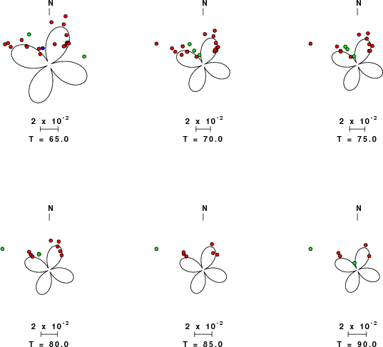
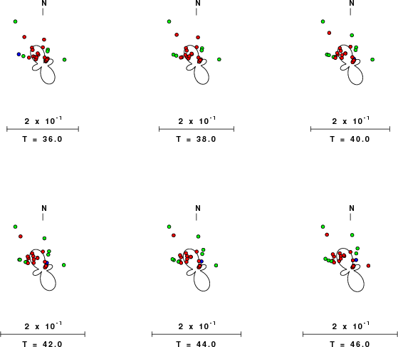
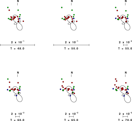
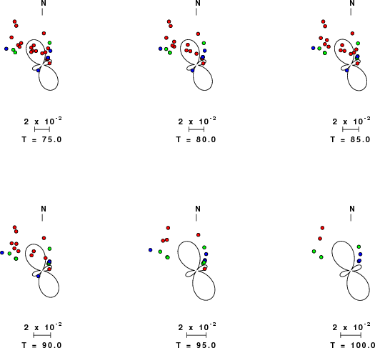
The following figure shows the stations used in the grid search for the best focal mechanism to fit the surface-wave spectral amplitudes of the Love and Rayleigh waves.
|
|
|
|
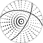
The surface-wave determined focal mechanism is shown here.
  NODAL PLANES


  STK=      30.00
  DIP=      69.99
 RAKE=      44.99

             OR

  STK=     281.12
  DIP=      48.37
 RAKE=     152.76


DEPTH = 9.0 km

Mw = 5.67
Best Fit 0.7159 - P-T axis plot gives solutions with FIT greater than FIT90
 |
The P-wave first motion data for focal mechanism studies are as follow:
Sta Az(deg) Dist(km) First motion
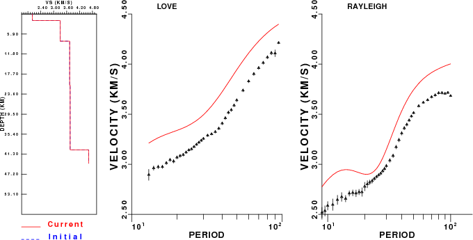
Surface wave analysis was performed using codes from Computer Programs in Seismology, specifically the multiple filter analysis program do_mft and the surface-wave radiation pattern search program srfgrd96.
Digital data were collected, instrument response removed and traces converted
to Z, R an T components. Multiple filter analysis was applied to the Z and T traces to obtain the Rayleigh- and Love-wave spectral amplitudes, respectively.
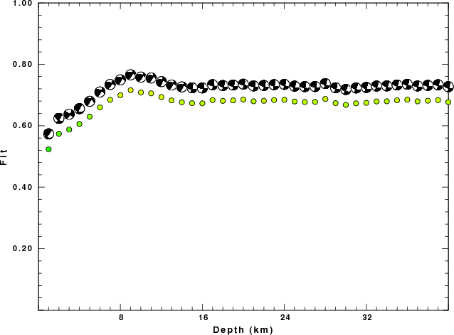
These were input to the search program which examined all depths between 1 and 25 km
and all possible mechanisms.
|
|
|
|
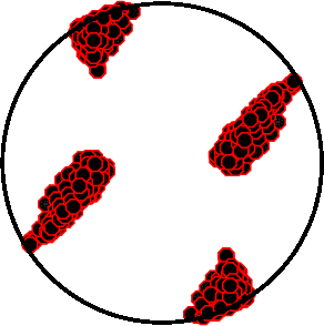
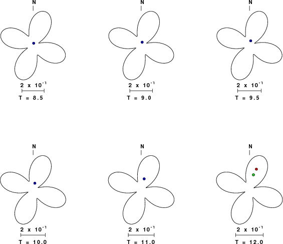
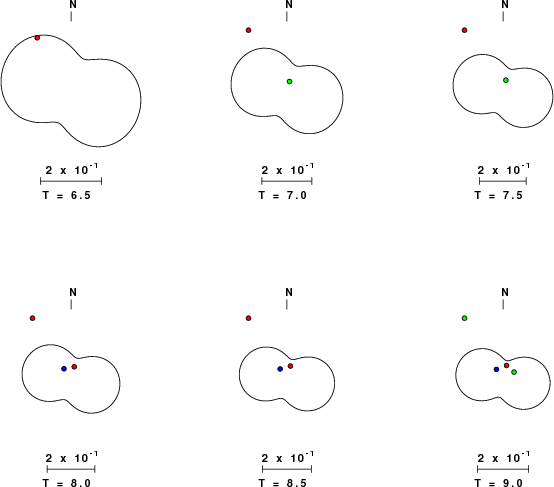
| Pressure-tension axis trends. Since the surface-wave spectra search does not distinguish between P and T axes and since there is a 180 ambiguity in strike, all possible P and T axes are plotted. First motion data and waveforms will be used to select the preferred mechanism. The purpose of this plot is to provide an idea of the possible range of solutions. The P and T-axes for all mechanisms with goodness of fit greater than 0.9 FITMAX (above) are plotted here. |
|
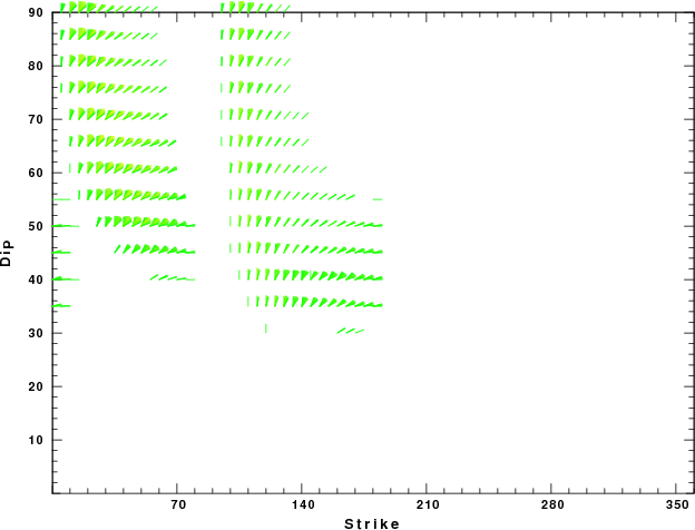
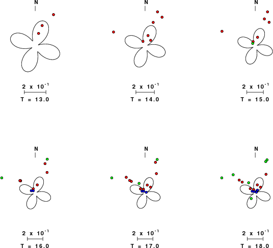
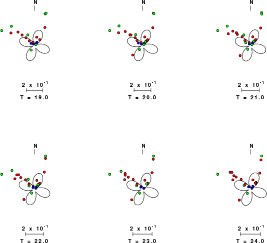
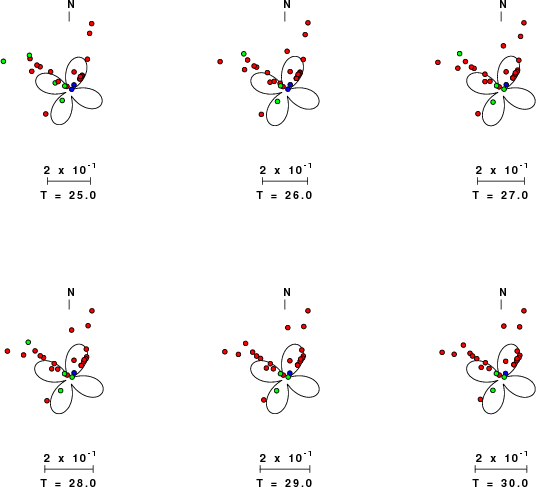
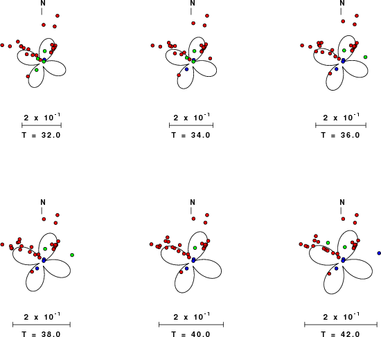
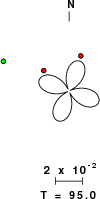
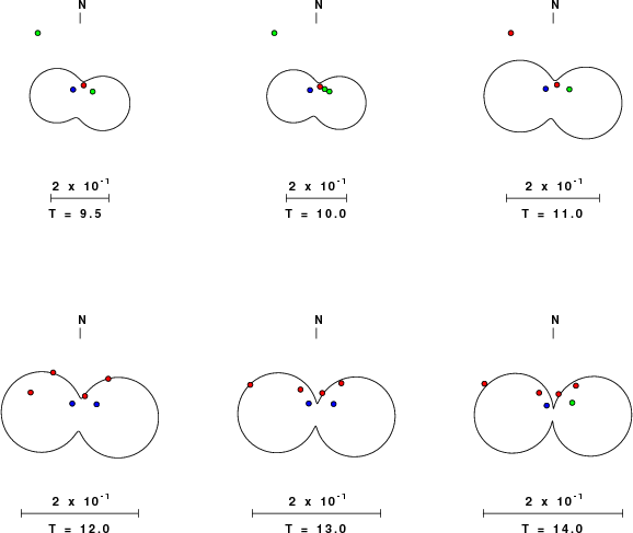
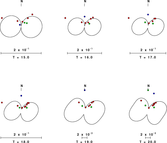
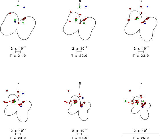
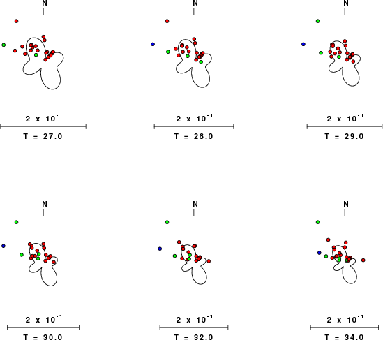
| Focal mechanism sensitivity at the preferred depth. The red color indicates a very good fit to the Love and Rayleigh wave radiation patterns. Each solution is plotted as a vector at a given value of strike and dip with the angle of the vector representing the rake angle, measured, with respect to the upward vertical (N) in the figure. Because of the symmetry of the spectral amplitude rediation patterns, only strikes from 0-180 degrees are sampled. |
The distribution of broadband stations with azimuth and distance is
Sta Az(deg)    Dist(km)
KRBR	   15	  346
ZHSF	   58	  567
NASN	  336	  709
SHGR	  312	  888
ASAO	  328	 1008
CHTH	  337	 1087
MRVT	    0	 1201
SNGE	  320	 1211
MAKU	  326	 1720
GNI	  328	 1785
MALT	  312	 2056
KSDI	  294	 2059
CSS	  298	 2318
AML	   40	 2338
EKS2	   38	 2382
UCH	   40	 2397
KZA	   42	 2435
KBK	   40	 2455
USP	   38	 2471
ULHL	   42	 2512
TKM2	   40	 2515
ANTO	  310	 2564
LAST	  295	 3022
IDI	  295	 3077
VOS	   20	 3125
BRVK	   19	 3135
GVD	  294	 3143
KURK	   30	 3268
ARU	    3	 3281
VTS	  309	 3421
LSA	   77	 3461
KIEV	  327	 3468
OBN	  339	 3495
KMBO	  216	 3690
DIVS	  310	 3723
TIP	  301	 3857
PSZ	  316	 3884
MBAR	  225	 4063
Since the analysis of the surface-wave radiation patterns uses only spectral amplitudes and because the surfave-wave radiation patterns have a 180 degree symmetry, each surface-wave solution consists of four possible focal mechanisms corresponding to the interchange of the P- and T-axes and a roation of the mechanism by 180 degrees. To select one mechanism, P-wave first motion can be used. This was not possible in this case because all the P-wave first motions were emergent ( a feature of the P-wave wave takeoff angle, the station location and the mechanism). The other way to select among the mechanisms is to compute forward synthetics and compare the observed and predicted waveforms.
The fits to the waveforms with the given mechanism are show below:

|
This figure shows the fit to the three components of motion (Z - vertical, R-radial and T - transverse). For each station and component, the observed traces is shown in red and the model predicted trace in blue. The traces represent filtered ground velocity in units of meters/sec (the peak value is printed adjacent to each trace; each pair of traces to plotted to the same scale to emphasize the difference in levels). Both synthetic and observed traces have been filtered using the SAC commands:
|
|
Should the national backbone of the USGS Advanced National Seismic System (ANSS) be implemented with an interstation separation of 300 km, it is very likely that an earthquake such as this would have been recorded at distances on the order of 100-200 km. This means that the closest station would have information on source depth and mechanism that was lacking here.
Dr. Harley Benz, USGS, provided the USGS USNSN digital data. The digital data used in this study were provided by Natural Resources Canada through their AUTODRM site http://www.seismo.nrcan.gc.ca/nwfa/autodrm/autodrm_req_e.php, and IRIS using their BUD interface
The WUS used for the waveform synthetic seismograms and for the surface wave eigenfunctions and dispersion is as follows:
MODEL.01
Model after     8 iterations
ISOTROPIC
KGS
FLAT EARTH
1-D
CONSTANT VELOCITY
LINE08
LINE09
LINE10
LINE11
      H(KM)   VP(KM/S)   VS(KM/S) RHO(GM/CC)         QP         QS       ETAP       ETAS      FREFP      FREFS
     1.9000     3.4065     2.0089     2.2150  0.302E-02  0.679E-02   0.00       0.00       1.00       1.00
     6.1000     5.5445     3.2953     2.6089  0.349E-02  0.784E-02   0.00       0.00       1.00       1.00
    13.0000     6.2708     3.7396     2.7812  0.212E-02  0.476E-02   0.00       0.00       1.00       1.00
    19.0000     6.4075     3.7680     2.8223  0.111E-02  0.249E-02   0.00       0.00       1.00       1.00
     0.0000     7.9000     4.6200     3.2760  0.164E-10  0.370E-10   0.00       0.00       1.00       1.00
Here we tabulate the reasons for not using certain digital data sets
DATE=Fri Aug 17 13:03:13 CDT 2007