
2006/04/17 02:44:05 39.57N 17.14E 10 4.3 Italy
USGS Felt map for this earthquake
USGS Felt reports page for Intermountain Western US
SLU Moment Tensor Solution
2006/04/17 02:44:05 39.57N 17.14E 10 4.3 Italy
Best Fitting Double Couple
Mo = 1.72e+23 dyne-cm
Mw = 4.79
Z = 30 km
Plane Strike Dip Rake
NP1 34 76 154
NP2 130 65 15
Principal Axes:
Axis Value Plunge Azimuth
T 1.72e+23 28 350
N 0.00e+00 61 188
P -1.72e+23 8 84
Moment Tensor: (dyne-cm)
Component Value
Mxx 1.28e+23
Mxy -4.29e+22
Mxz 6.70e+22
Myy -1.62e+23
Myz -3.54e+22
Mzz 3.41e+22
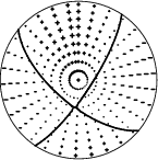
##############
####### ############
########## T ############---
########### ############----
-##########################-------
---########################---------
-----#######################----------
------######################------------
-------####################-----------
----------#################------------ P
-----------###############-------------
-------------############-----------------
---------------########-------------------
----------------#####-------------------
------------------##--------------------
-----------------###------------------
---------------#######--------------
------------#############---------
--------######################
-----#######################
######################
##############
Harvard Convention
Moment Tensor:
R T F
3.41e+22 6.70e+22 3.54e+22
6.70e+22 1.28e+23 4.29e+22
3.54e+22 4.29e+22 -1.62e+23
Details of the solution is found at
http://www.eas.slu.edu/Earthquake_Center/NEW/20060417024405/index.html
|
The focal mechanism was determined using broadband seismic waveforms. The location of the event and the station distribution are given in Figure 1.
|
|
|
|
      STK = 130
      DIP = 65
     RAKE = 15
       MW = 4.79
       HS = 30
The solution given here is from waveform inversion of regional vaeforms from the INGV digital seismic stations.
The program wvfgrd96 was used with good traces observed at short distance to determine the focal mechanism, depth and seismic moment. This technique requires a high quality signal and well determined velocity model for the Green functions. To the extent that these are the quality data, this type of mechanism should be preferred over the radiation pattern technique which requires the separate step of defining the pressure and tension quadrants and the correct strike.
The observed and predicted traces are filtered using the following gsac commands:
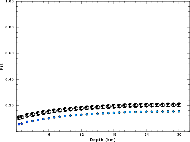
hp c 0.02 3
lp c 0.04 3
The results of this grid search from 0.5 to 19 km depth are as follow:
           DEPTH  STK   DIP  RAKE   MW    FIT
WVFGRD96    0.5   120    35    10   4.46 0.0556
WVFGRD96    1.0   120    55    15   4.39 0.0600
WVFGRD96    2.0   120    50    15   4.48 0.0738
WVFGRD96    3.0   110    55    -5   4.49 0.0806
WVFGRD96    4.0   110    55    -5   4.52 0.0875
WVFGRD96    5.0   110    60   -10   4.54 0.0948
WVFGRD96    6.0   110    55   -10   4.57 0.1007
WVFGRD96    7.0   110    55   -15   4.59 0.1079
WVFGRD96    8.0   110    55   -15   4.62 0.1132
WVFGRD96    9.0   110    55   -15   4.63 0.1181
WVFGRD96   10.0   110    55   -20   4.64 0.1220
WVFGRD96   11.0   110    55   -20   4.65 0.1256
WVFGRD96   12.0   110    55   -20   4.66 0.1283
WVFGRD96   13.0   110    55   -20   4.67 0.1312
WVFGRD96   14.0   115    60   -15   4.66 0.1342
WVFGRD96   15.0   115    60   -10   4.67 0.1365
WVFGRD96   16.0   115    60   -10   4.68 0.1392
WVFGRD96   17.0   115    60   -10   4.69 0.1408
WVFGRD96   18.0   115    65   -10   4.69 0.1428
WVFGRD96   19.0   120    65   -10   4.69 0.1454
WVFGRD96   20.0   120    65   -10   4.70 0.1477
WVFGRD96   21.0   120    65   -10   4.73 0.1493
WVFGRD96   22.0   120    65   -10   4.73 0.1500
WVFGRD96   23.0   120    65   -10   4.74 0.1512
WVFGRD96   24.0   120    65   -10   4.75 0.1521
WVFGRD96   25.0   120    65   -10   4.75 0.1521
WVFGRD96   26.0   120    65    -5   4.76 0.1527
WVFGRD96   27.0   120    65    -5   4.77 0.1531
WVFGRD96   28.0   130    65    15   4.77 0.1531
WVFGRD96   29.0   130    65    15   4.78 0.1538
WVFGRD96   30.0   130    65    15   4.79 0.1542
The best solution is
WVFGRD96 30.0 130 65 15 4.79 0.1542
The mechanism correspond to the best fit is
|
|
|
The best fit as a function of depth is given in the following figure:
|
|
|
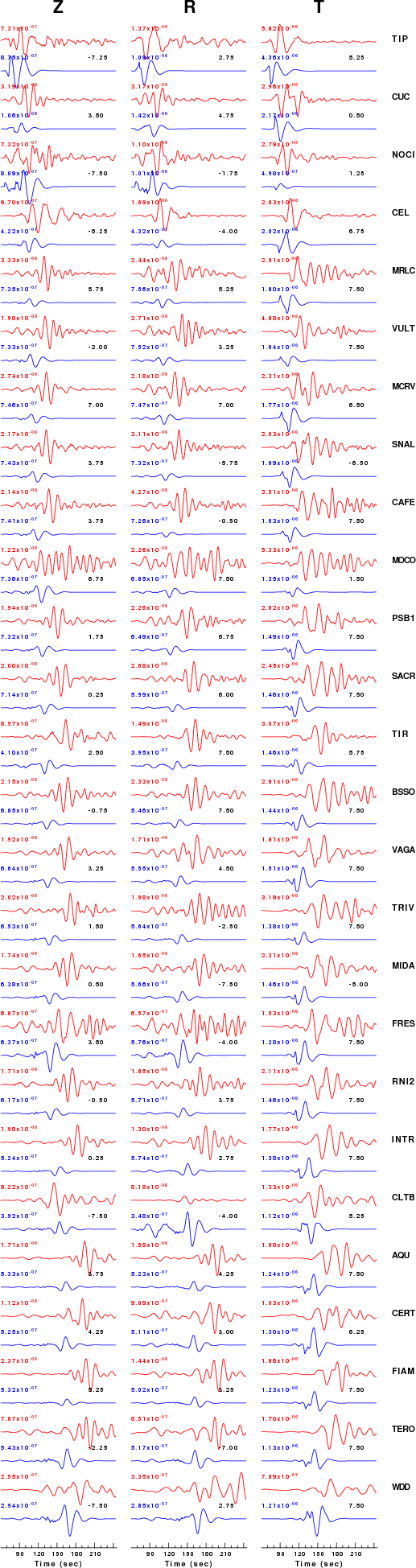
The comparison of the observed and predicted waveforms is given in the next figure. The red traces are the observed and the blue are the predicted. Each observed-predicted componnet is plotted to the same scale and peak amplitudes are indicated by the numbers to the left of each trace. The number in black at the rightr of each predicted traces it the time shift required for maximum correlation between the observed and predicted traces. This time shift is required because the synthetics are not computed at exactly the same distance as the observed and because the velocity model used in the predictions may not be perfect. A positive time shift indicates that the prediction is too fast and should be delayed to match the observed trace (shift to the right in this figure). A negative value indicates that the prediction is too slow. The bandpass filter used in the processing and for the display was
hp c 0.02 3
lp c 0.04 3
|
|
|
|
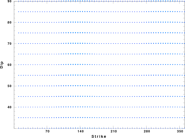
| Focal mechanism sensitivity at the preferred depth. The red color indicates a very good fit to thewavefroms. Each solution is plotted as a vector at a given value of strike and dip with the angle of the vector representing the rake angle, measured, with respect to the upward vertical (N) in the figure. |
The P-wave first motion data for focal mechanism studies are as follow:
Sta Az(deg)    Dist(km)   First motion
TIP       217   54 iP_C
CUC       293  123 eP_+
NOCI      357  136 iP_C
AMUR      343  155 iP_C
CEL       217  181 eP_+
MRLC      314  193 iP_C
VULT      320  201 iP_C
MCRV      309  215 iP_C
SNAL      313  223 eP_X
CAFE      316  229 iP_C
MOCO      321  261 eP_X
PSB1      314  270 iP_C
SACR      315  290 iP_C
TIR        49  304 eP_X
BSSO      316  308 iP_C
VAGA      311  320 eP_+
TRIV      319  328 iP_C
MIDA      314  336 iP_C
FRES      323  339 iP_C
RNI2      314  346 iP_C
INTR      316  385 iP_C
CLTB      238  407 eP_X
CERT      308  439 iP_C
AQU       316  441 iP_C
TERO      320  451 iP_C
FIAM      313  452 iP_C
WDD       210  471 eP_X
The follwoing stations were not used because of excessive low frequency noise in the deconvolved waveforms: AMUR, GIUL, RNI2, SNAL, TRIV