2005/10/30 19:09:46 38.53 15.93E 24 3.6 Italy
USGS Felt map for this earthquake
USGS Felt reports page for Intermountain Western US
 SLU Moment Tensor Solution
 2005/10/30 19:09:46 38.53 15.93E 24 3.6 Italy

 Best Fitting Double Couple
    Mo = 2.45e+21 dyne-cm
    Mw = 3.56
    Z  = 14 km
     Plane   Strike  Dip  Rake
      NP1       45    59   -106
      NP2      255    35   -65
 Principal Axes:
   Axis    Value   Plunge  Azimuth
     T   2.45e+21     12     147
     N   0.00e+00     14      54
     P  -2.45e+21     71     277


 Moment Tensor: (dyne-cm)
    Component  Value
       Mxx     1.65e+21
       Mxy    -1.04e+21
       Mxz    -5.15e+20
       Myy     4.38e+20
       Myz     1.02e+21
       Mzz    -2.09e+21


                     ##############
                 ######################
              ############################
             ################----##########
           ##########-------------------###--
          ########----------------------------
         ######---------------------------####-
        #####-----------------------------#####-
        ####-----------------------------#######
       ####-----------   ---------------#########
       ###------------ P --------------##########
       ##-------------   -------------###########
       #----------------------------#############
        ---------------------------#############
        -------------------------###############
         ----------------------################
          ------------------##################
           --------------####################
             -------################   ####
              ###################### T ###
                 ###################
                     ##############


 Harvard Convention
 Moment Tensor:
      R          T          F
 -2.09e+21  -5.15e+20  -1.02e+21
 -5.15e+20   1.65e+21   1.04e+21
 -1.02e+21   1.04e+21   4.38e+20


Details of the solution is found at

http://www.eas.slu.edu/Earthquake_Center/NEW/20051030190946/index.html
|
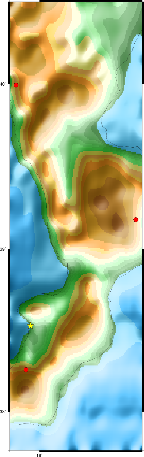
The focal mechanism was determined using broadband seismic waveforms. The location of the event and the station distribution are given in Figure 1.
|
|
|
|
      STK = 255
      DIP = 35
     RAKE = -65
       MW = 3.56
       HS = 14
The solution given here is from waveform inversion of regional vaeforms from the INGV digital seismic stations.
The program wvfgrd96 was used with good traces observed at short distance to determine the focal mechanism, depth and seismic moment. This technique requires a high quality signal and well determined velocity model for the Green functions. To the extent that these are the quality data, this type of mechanism should be preferred over the radiation pattern technique which requires the separate step of defining the pressure and tension quadrants and the correct strike.
The observed and predicted traces are filtered using the following gsac commands:
hp c 0.02 3
lp c 0.05 3
The results of this grid search from 0.5 to 19 km depth are as follow:
           DEPTH  STK   DIP  RAKE   MW    FIT
WVFGRD96    0.5   170    40    80   3.37 0.4325
WVFGRD96    1.0   305    85    10   3.11 0.3587
WVFGRD96    2.0   160    45    70   3.44 0.4571
WVFGRD96    3.0   160    45    75   3.44 0.4250
WVFGRD96    4.0   300    85    60   3.37 0.4419
WVFGRD96    5.0   300    85    55   3.38 0.4981
WVFGRD96    6.0   115    90   -55   3.39 0.5350
WVFGRD96    7.0   105    80   -55   3.39 0.5634
WVFGRD96    8.0   105    80   -55   3.42 0.5883
WVFGRD96    9.0   250    25   -70   3.53 0.6169
WVFGRD96   10.0   240    30   -85   3.52 0.6487
WVFGRD96   11.0   250    30   -70   3.55 0.6755
WVFGRD96   12.0   260    30   -55   3.57 0.6928
WVFGRD96   13.0   250    35   -70   3.56 0.7056
WVFGRD96   14.0   255    35   -65   3.56 0.7098
WVFGRD96   15.0   265    35   -50   3.59 0.7046
WVFGRD96   16.0   255    40   -65   3.56 0.6989
WVFGRD96   17.0   265    40   -50   3.59 0.6901
WVFGRD96   18.0   250    45   -70   3.56 0.6743
WVFGRD96   19.0   260    45   -55   3.58 0.6670
WVFGRD96   20.0   265    45   -50   3.60 0.6572
WVFGRD96   21.0   260    45   -55   3.63 0.6575
WVFGRD96   22.0   250    50   -70   3.61 0.6477
WVFGRD96   23.0   255    50   -65   3.62 0.6422
WVFGRD96   24.0   260    50   -55   3.64 0.6340
WVFGRD96   25.0   265    50   -50   3.65 0.6223
WVFGRD96   26.0   250    55   -70   3.62 0.6100
WVFGRD96   27.0   255    55   -65   3.63 0.5987
WVFGRD96   28.0   265    55   -50   3.65 0.5884
WVFGRD96   29.0   275    55   -35   3.69 0.5766
WVFGRD96   30.0   305    90    30   3.65 0.5666
The best solution is
WVFGRD96 14.0 255 35 -65 3.56 0.7098
The mechanism correspond to the best fit is
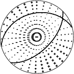
|
|
|
The best fit as a function of depth is given in the following figure:
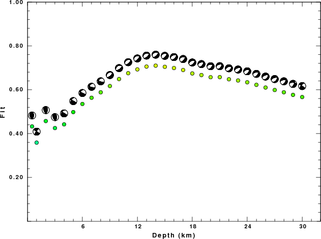
|
|
|
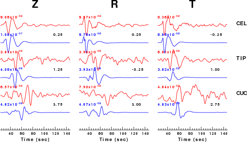
The comparison of the observed and predicted waveforms is given in the next figure. The red traces are the observed and the blue are the predicted. Each observed-predicted componnet is plotted to the same scale and peak amplitudes are indicated by the numbers to the left of each trace. The number in black at the rightr of each predicted traces it the time shift required for maximum correlation between the observed and predicted traces. This time shift is required because the synthetics are not computed at exactly the same distance as the observed and because the velocity model used in the predictions may not be perfect. A positive time shift indicates that the prediction is too fast and should be delayed to match the observed trace (shift to the right in this figure). A negative value indicates that the prediction is too slow. The bandpass filter used in the processing and for the display was
hp c 0.02 3
lp c 0.05 3
|
|
|
|
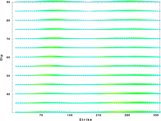
| Focal mechanism sensitivity at the preferred depth. The red color indicates a very good fit to thewavefroms. Each solution is plotted as a vector at a given value of strike and dip with the angle of the vector representing the rake angle, measured, with respect to the upward vertical (N) in the figure. |
The P-wave first motion data for focal mechanism studies are as follow:
Sta Az(deg)    Dist(km)   First motion
CEL       186   30 iP_C
TIP        45  102 eP_X
CUC       357  163 eP_X
MRLC      351  250 eP_X
MCRV      346  259 eP_X
NOCI       21  269 eP_X
AMUR       12  270 eP_+
VULT      354  271 eP_X
SNAL      347  273 eP_X
CAFE      348  284 eP_X
PSB1      343  314 eP_X
WDD       203  321 eP_X
The follwoing stations were not used because of excessive low frequency noise in the deconvolved waveforms: AMUR, GIUL, RNI2, SNAL, TRIV