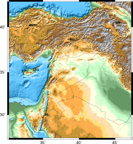
Stations used for waveform inversion
2005/05/24 09:40:12 35.37N 39.21E 10 4.6 Syria
USGS Felt map for this earthquake
USGS Felt reports page for Syria
 SLU Moment Tensor Solution
 2005/05/24 09:40:12 35.37N 39.21E 10 4.6 Syria

 Best Fitting Double Couple
    Mo = 1.66e+22 dyne-cm
    Mw = 4.08
    Z  = 25 km
     Plane   Strike  Dip  Rake
      NP1      330    73   -148
      NP2      230    60   -20
 Principal Axes:
   Axis    Value   Plunge  Azimuth
     T   1.66e+22      8      98
     N   0.00e+00     54     356
     P  -1.66e+22     34     194


 Moment Tensor: (dyne-cm)
    Component  Value
       Mxx    -1.04e+22
       Mxy    -4.77e+21
       Mxz     7.19e+21
       Myy     1.53e+22
       Myz     4.15e+21
       Mzz    -4.92e+21


                     --------------
                 ##--------------------
              #######---------------------
             ##########--------------------
           ##############---------###########
          ################---#################
         #################--###################
        ################-----###################
        ##############--------##################
       #############-----------##################
       ###########---------------################
       ##########----------------#############
       #########------------------############ T
        #######--------------------###########
        ######----------------------############
         ####------------------------##########
          ##-------------------------#########
           #-----------   ------------#######
             ---------- P ------------#####
              ---------   ------------####
                 ---------------------#
                     --------------


 Harvard Convention
 Moment Tensor:
      R          T          F
 -4.92e+21   7.19e+21  -4.15e+21
  7.19e+21  -1.04e+22   4.77e+21
 -4.15e+21   4.77e+21   1.53e+22


Details of the solution is found at

http://www.eas.slu.edu/Earthquake_Center/MECH.NA/20050524094012/index.html
|
      STK = 230
      DIP = 60
     RAKE = -20
       MW = 4.08
       HS = 25
The depth is not well determined. Both techniques give the same moment and similar directions fo the P- and T-axes. The addition of regional broadband recordings would be useful.
The program wvfgrd96 was used with good traces observed at short distance to determine the focal mechanism, depth and seismic moment. This technique requires a high quality signal and well determined velocity model for the Green functions. To the extent that these are the quality data, this type of mechanism should be preferred over the radiation pattern technique which requires the separate step of defining the pressure and tension quadrants and the correct strike.
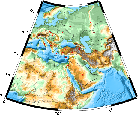
The stations used in the inversion are given in the next figure.
|
Stations used for waveform inversion |
The observed and predicted traces are filtered using the following gsac commands:
hp c 0.01 3
lp c 0.04 3
The results of this grid search from 0.5 to 19 km depth are as follow:
           DEPTH  STK   DIP  RAKE   MW    FIT
WVFGRD96    0.5   240    10     0   4.21 0.3287
WVFGRD96    1.0   240    20     0   4.04 0.3562
WVFGRD96    2.0   240    25     0   4.04 0.3935
WVFGRD96    3.0   240    50     0   3.90 0.3949
WVFGRD96    4.0   240    75    -5   3.88 0.4260
WVFGRD96    5.0   240    80    -5   3.90 0.4348
WVFGRD96    6.0   245    90    -5   3.96 0.4634
WVFGRD96    7.0   245    80   -20   3.99 0.4706
WVFGRD96    8.0   245    80   -20   4.02 0.4931
WVFGRD96    9.0   245    80   -20   4.03 0.4922
WVFGRD96   10.0   245    80   -20   4.04 0.4830
WVFGRD96   11.0   210    70    30   4.01 0.4845
WVFGRD96   12.0   245    80   -20   4.05 0.4809
WVFGRD96   13.0   240    60   -20   4.04 0.4973
WVFGRD96   14.0   240    65   -20   4.05 0.5108
WVFGRD96   15.0   235    60   -20   4.03 0.5215
WVFGRD96   16.0   235    60   -20   4.03 0.5379
WVFGRD96   17.0   235    60   -20   4.03 0.5484
WVFGRD96   18.0   240    65   -15   4.06 0.5576
WVFGRD96   19.0   240    65   -15   4.07 0.5653
WVFGRD96   20.0   235    65   -15   4.05 0.5696
WVFGRD96   21.0   235    60   -20   4.08 0.5792
WVFGRD96   22.0   230    60   -20   4.07 0.5844
WVFGRD96   23.0   230    60   -20   4.08 0.5872
WVFGRD96   24.0   230    60   -20   4.08 0.5864
WVFGRD96   25.0   230    60   -20   4.08 0.5885
WVFGRD96   26.0   230    60   -20   4.09 0.5859
WVFGRD96   27.0   230    60   -20   4.09 0.5837
WVFGRD96   28.0   225    60   -20   4.08 0.5834
WVFGRD96   29.0   225    60   -20   4.09 0.5784
WVFGRD96   30.0   230    65   -15   4.11 0.5759
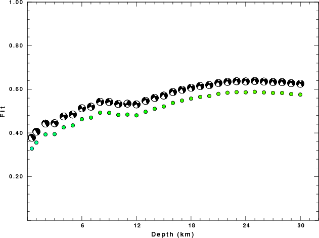
The best solution is
WVFGRD96 25.0 230 60 -20 4.08 0.5885
The mechanism correspond to the best fit is
|
|
|
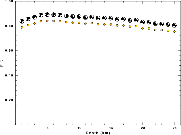
The best fit as a function of depth is given in the following figure:
|
|
|
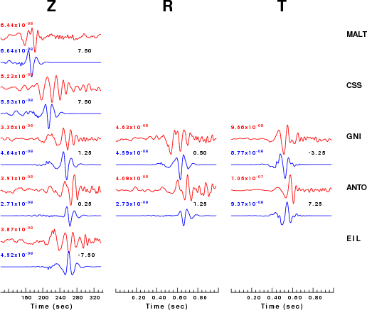
The comparison of the observed and predicted waveforms is given in the next figure. The red traces are the observed and the blue are the predicted. Each observed-predicted componnet is plotted to the same scale and peak amplitudes are indicated by the numbers to the left of each trace. The number in black at the rightr of each predicted traces it the time shift required for maximum correlation between the observed and predicted traces. This time shift is required because the synthetics are not computed at exactly the same distance as the observed and because the velocity model used in the predictions may not be perfect. A positive time shift indicates that the prediction is too fast and should be delayed to match the observed trace (shift to the right in this figure). A negative value indicates that the prediction is too slow. The bandpass filter used in the processing and for the display was
hp c 0.01 3
lp c 0.04 3
|
|
|
|
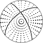
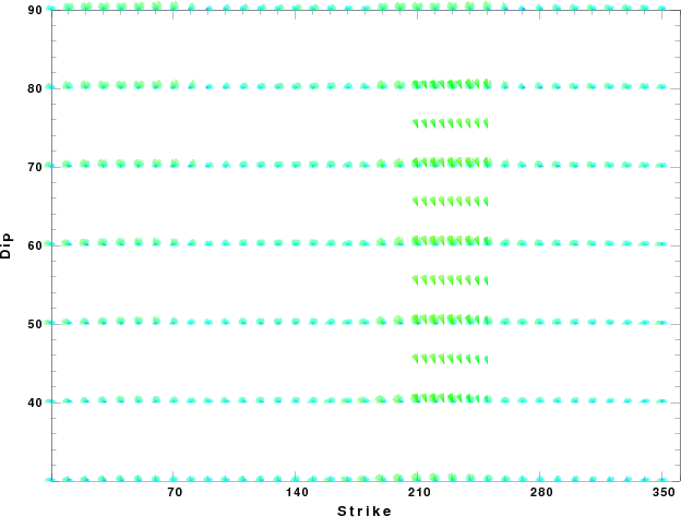
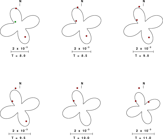
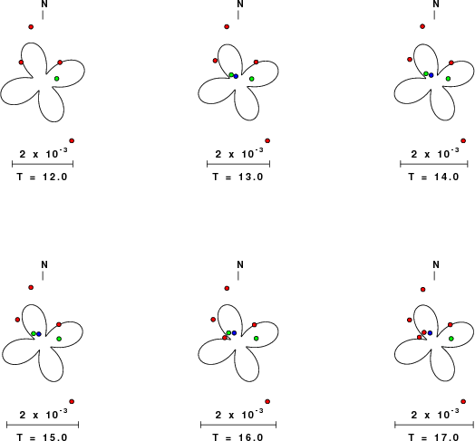
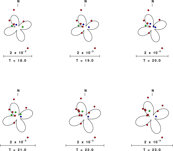
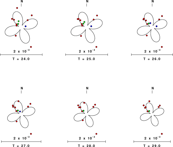
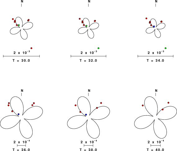
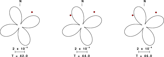
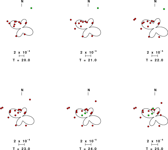
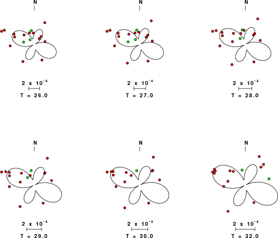
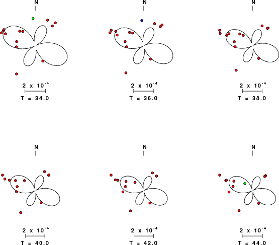
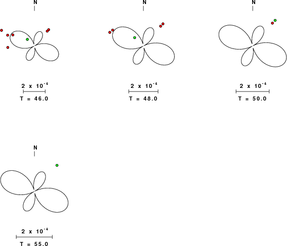
| Focal mechanism sensitivity at the preferred depth. The red color indicates a very good fit to thewavefroms. Each solution is plotted as a vector at a given value of strike and dip with the angle of the vector representing the rake angle, measured, with respect to the upward vertical (N) in the figure. |
The following figure shows the stations used in the grid search for the best focal mechanism to fit the surface-wave spectral amplitudes of the Love and Rayleigh waves.
|
|
|
The surface-wave determined focal mechanism is shown here.
  NODAL PLANES


  STK=     244.24
  DIP=      79.45
 RAKE=     -45.99

             OR

  STK=     344.98
  DIP=      45.00
 RAKE=    -164.99


DEPTH = 5.0 km

Mw = 4.10
Best Fit 0.8410 - P-T axis plot gives solutions with FIT greater than FIT90
 |
The P-wave first motion data for focal mechanism studies are as follow:
Sta Az(deg)    Dist(km)   First motion
MALT      348  334 eP_-
CSS       267  537 eP_X
GNI        41  720 eP_X
EIL       213  748 eP_X
ANTO      313  755 eP_X
Surface wave analysis was performed using codes from Computer Programs in Seismology, specifically the multiple filter analysis program do_mft and the surface-wave radiation pattern search program srfgrd96.
The velocity model used for the search is a modified Utah model .
Digital data were collected, instrument response removed and traces converted
to Z, R an T components. Multiple filter analysis was applied to the Z and T traces to obtain the Rayleigh- and Love-wave spectral amplitudes, respectively.
These were input to the search program which examined all depths between 1 and 25 km
and all possible mechanisms.
|
|
|
|
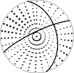
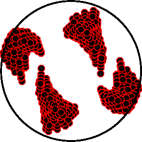
| Pressure-tension axis trends. Since the surface-wave spectra search does not distinguish between P and T axes and since there is a 180 ambiguity in strike, all possible P and T axes are plotted. First motion data and waveforms will be used to select the preferred mechanism. The purpose of this plot is to provide an idea of the possible range of solutions. The P and T-axes for all mechanisms with goodness of fit greater than 0.9 FITMAX (above) are plotted here. |
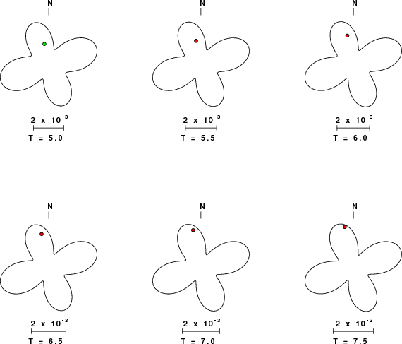
|
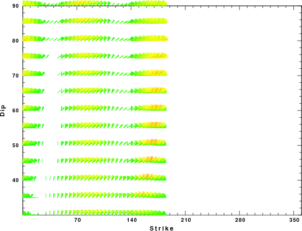
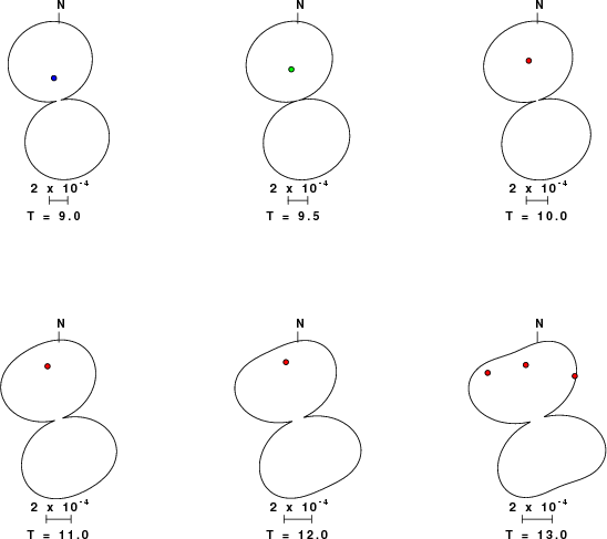
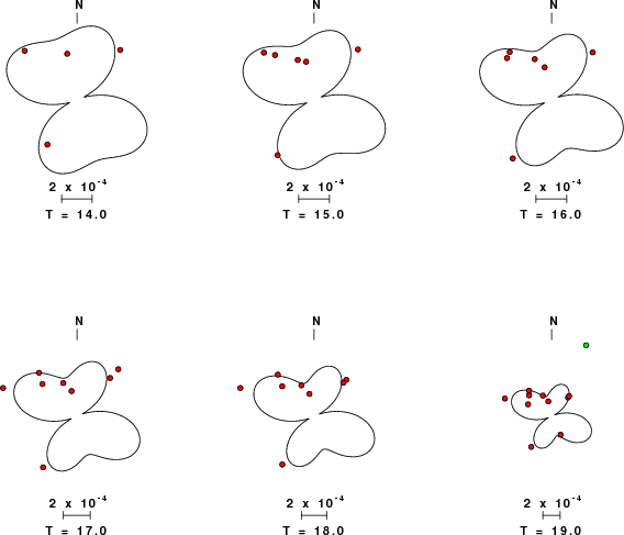
| Focal mechanism sensitivity at the preferred depth. The red color indicates a very good fit to the Love and Rayleigh wave radiation patterns. Each solution is plotted as a vector at a given value of strike and dip with the angle of the vector representing the rake angle, measured, with respect to the upward vertical (N) in the figure. Because of the symmetry of the spectral amplitude rediation patterns, only strikes from 0-180 degrees are sampled. |
Sta Az(deg)    Dist(km)
MALT	  348	  334
CSS	  267	  537
GNI	   41	  720
EIL	  214	  748
ANTO	  313	  755
ISP	  292	  825
APE	  283	 1243
RAYN	  154	 1447
ABKT	   75	 1711
TIR	  297	 1812
KIEV	  338	 1883
PSZ	  317	 2118
CUC	  291	 2120
OBN	  356	 2204
CII	  296	 2273
ABKAR	   41	 2288
MORC	  319	 2377
DPC	  319	 2480
ARU	   26	 2760
SENIN	  304	 2928
Since the analysis of the surface-wave radiation patterns uses only spectral amplitudes and because the surfave-wave radiation patterns have a 180 degree symmetry, each surface-wave solution consists of four possible focal mechanisms corresponding to the interchange of the P- and T-axes and a roation of the mechanism by 180 degrees. To select one mechanism, P-wave first motion can be used. This was not possible in this case because all the P-wave first motions were emergent ( a feature of the P-wave wave takeoff angle, the station location and the mechanism). The other way to select among the mechanisms is to compute forward synthetics and compare the observed and predicted waveforms.
The velocity model used for the waveform fit is a modified Utah model .
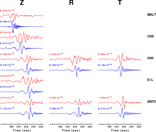
The fits to the waveforms with the given mechanism are show below:
|
This figure shows the fit to the three components of motion (Z - vertical, R-radial and T - transverse). For each station and component, the observed traces is shown in red and the model predicted trace in blue. The traces represent filtered ground velocity in units of meters/sec (the peak value is printed adjacent to each trace; each pair of traces to plotted to the same scale to emphasize the difference in levels). Both synthetic and observed traces have been filtered using the SAC commands:
hp c 0.01 3
lp c 0.04 3
|
|
Should the national backbone of the USGS Advanced National Seismic System (ANSS) be implemented with an interstation separation of 300 km, it is very likely that an earthquake such as this would have been recorded at distances on the order of 100-200 km. This means that the closest station would have information on source depth and mechanism that was lacking here.
Dr. Harley Benz, USGS, provided the USGS USNSN digital data. The digital data used in this study were provided by Natural Resources Canada through their AUTODRM site http://www.seismo.nrcan.gc.ca/nwfa/autodrm/autodrm_req_e.php, and IRIS using their BUD interface
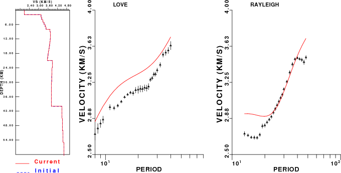
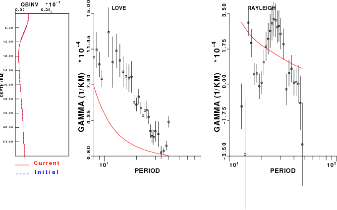
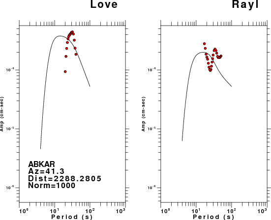
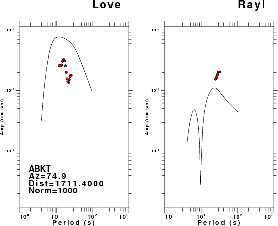
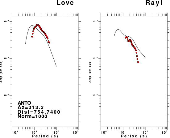
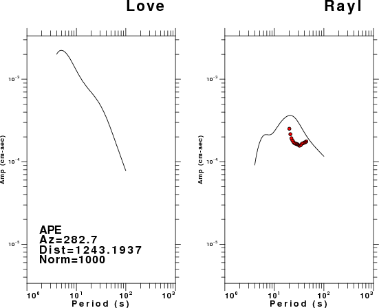
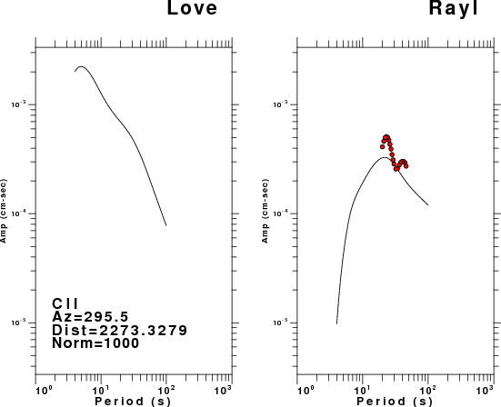
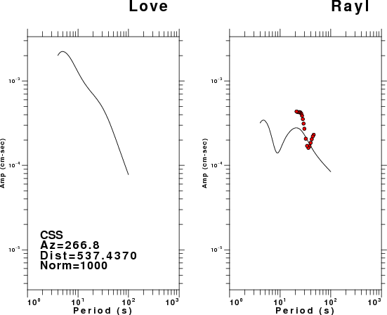
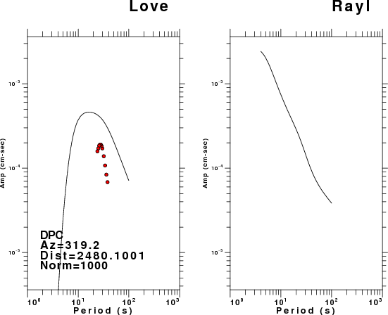
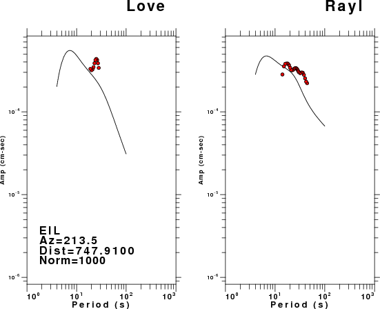
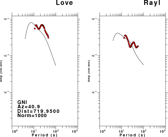
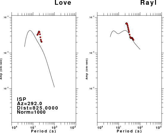
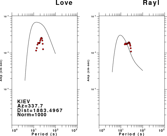
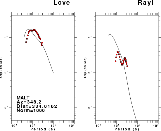
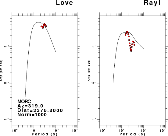
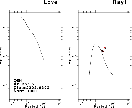
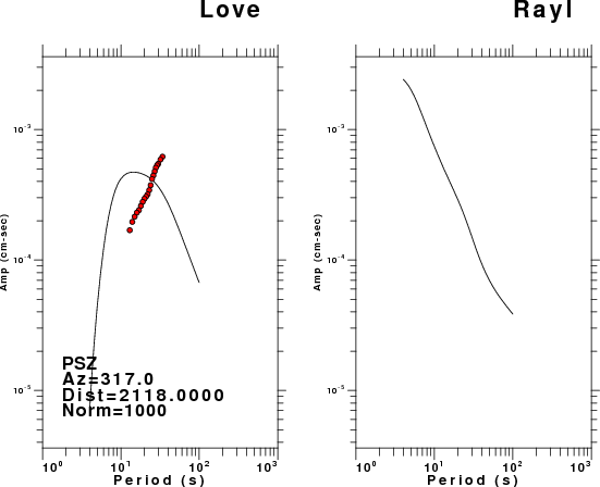
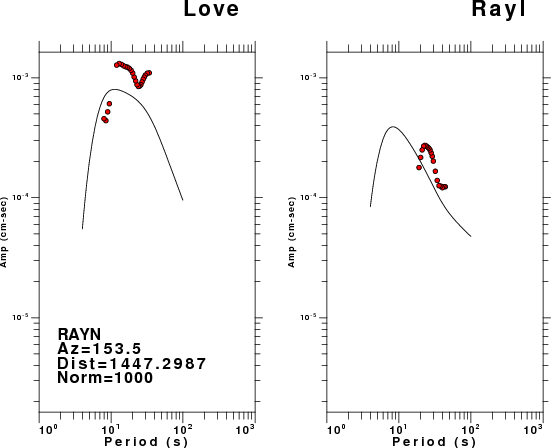
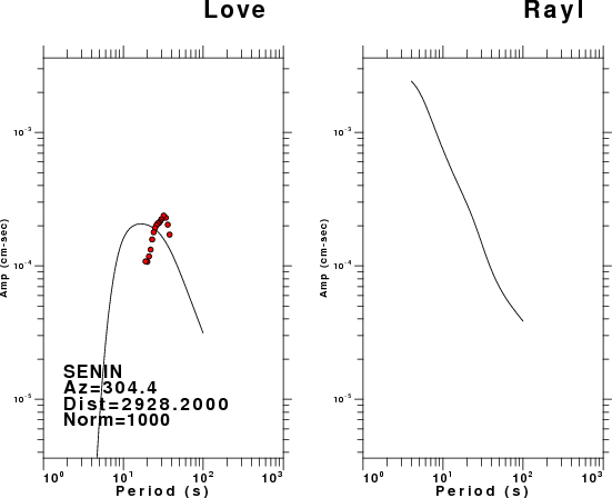
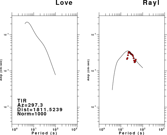
The figures below show the observed spectral amplitudes (units of cm-sec) at each station and the
theoretical predictions as a function of period for the mechanism given above. The modified Utah model earth model
was used to define the Green's functions. For each station, the Love and Rayleigh wave spectrail amplitudes are plotted with the same scaling so that one can get a sense fo the effects of the effects of the focal mechanism and depth on the excitation of each.
 |
 |
 |
 |
 |
 |
 |
 |
 |
 |
 |
 |
 |
 |
 |
 |
 |
 |
 |
 |
Here we tabulate the reasons for not using certain digital data sets
The following stations did not have a valid response files: